Logistic regression and support vector machines are widely used supervised learning models that give us a fast and efficient way of classifying new data based on a training set of classified, old data. While they appear similar, and often yield comparable results, they work in fundamentally different ways and both have their specificities.
Logistic regression, for a start, provides us with what we call a probabilistic model: applying that model to an unclassified entry yields the probability that it belongs to the class in question. In other terms: \(h(\vec{x}) = \frac{1}{1 + e^{\large – \vec{\theta} \cdot \vec{x}}} = P(y = 1)\), where \(h(\vec{x})\) is the hypothesis, \(\vec{\theta}\) the computed parameters, \(\vec{x}\) an entry and \(y\) the actual classification (unknown) of that entry.
But then, in cases where a categorization is always required, it is common for engineers and data scientists to assign \(\vec{x}\) to the class with the highest probability, even if it’s not very high, that is:
As the logistic function is monotonically increasing, this correponds to:

This is, in fact, the exact hypothesis of a support vector machine (only with a different \(\vec{\theta}\)), which directly yields this deterministic prediction without going through the probability stage. It is, however, possible to obtain an equivalent probability using Platt scaling, which means that at this point, the two models are very similar.
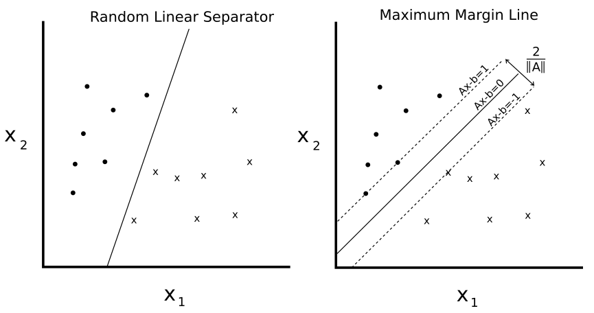
In the end, the main difference between them lies in the way they are trained. Support vector machines are what we call a large margin classifier, and they work by finding the optimal separating hyperplane for the data they are provided: that is, the one that maximizes the distance from it to the nearest data point on each side.
This training is achieved through the minimization of different cost functions. For logistic regression, the cost function can be expressed as the following:
(Note: the last term is used to prevent the model from overfitting, that is performing very well on the training set but failing to predict new entries. This technique is known as regularization, and can be adjusted with the parameter \(\lambda\). We are using the \(L^2\) norm here, but it is also possible to use the \(L^1\) norm or a linear combination of both.)
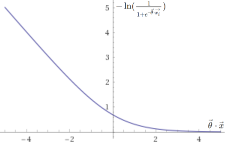
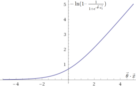
The cost function above is in fact based on two sub-functions, one that is used if the entry is positive (\(y = 1\)), \(– \ln(h(\vec{x}))\), and another if it is negative (\(y = 0\)), \(-\ln(1 – h(\vec{x}))\). They are plotted below.
Support vector machines, on the other hand, are trained by minimizing the following cost function:
(Note: A different notation is traditionally used for support vector machines, but I’ll stick to this one for the sake of comparison.)
The two corresponding sub-functions are plotted below:
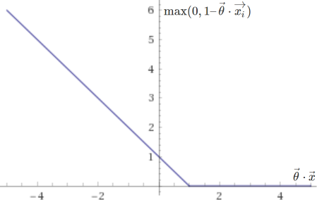
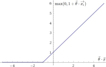
They are very similar to the ones used in logistic regression, except that they end more abruptly, placing no penalty on values of \(\vec{\theta} \cdot \vec{x}\) greater than \(1\) if \(y = 1\), or smaller than \(-1\) if \(y = 0\). This clear delimitation allows support vector machines to separate data with as high a margin as possible. Note that with \(\lambda\) very small (little to no regularization), this approach will be too sensitive to outliers and may not yield a truly optimal result.
But in the end, the most important difference beween logistic regression and support vector machines is how they work with kernels. Kernels are very useful when the data is not linearly separable: they allow us to map our entries (\(\in \mathbb R^{n}\)) to a new set of higher-dimensional entries (\(\in \mathbb R ^{m}\)) which can now be separated by an \(m – 1\)-dimensional hyperplane. A common example is the radial basis function kernel, which maps each entry in the data set to a decreasing function of the squared Euclidean distance between itself and each other entry: the associated kernel function is \(K(\vec{x_1}, \vec{x_2}) = \exp\left(-\frac{\|\vec{x_1} – \vec{x_2}\|^2}{2\sigma^2}\right)\). A wide variety of kernels exist, from polynomial to string kernels (useful for text inputs).
Kernels can be used with pretty much every machine learning algorithm, but they are particularly efficient with support vector machines. This is because it’s possible to use sequential minimal optimization, an algorithm that partitions the training problem into smaller ones that can be solved analytically, in their implementation. This speeds up training significantly.
Now what about the implementation? Both logistic regression and SVMs are supported by MLlib. A simple logistic regression can be implemented as follows:
|
1 2 3 4 5 6 7 8 9 10 11 12 13 |
// Load training data val training = spark.read.format("libsvm").load("data/mllib/sample_libsvm_data.txt") val logisticRegression = new LogisticRegression() .setMaxIter(10) .setRegParam(0.3) .setElasticNetParam(0.8) // Fit the model val logisticRegressionModel = logisticRegression.fit(training) // Print the coefficients and intercept for logistic regression println(s"Coefficients: ${logisticRegressionModel.coefficients} Intercept: ${logisticRegressionModel.intercept}") |
(Note: setRegParam sets the regularization parameter \(\lambda\), while setElasticNetParam sets the mix between the use of the \(L^1\) and \(L^2\) norms, from 0 for \(L^2\) to 1 for \(L^1\).)
And a support vector machine (with gradient descent) as the following:
|
1 2 3 4 5 6 7 8 9 |
// Load training data val training = spark.read.format("libsvm").load("data/mllib/sample_libsvm_data.txt") // Run training algorithm to build the model val numIterations = 100 val svmModel = SVMWithSGD.train(training, numIterations) // Print the weights and intercept for the support vector machine println(s"Weights: ${svmModel.weights} Intercept: ${svmModel.intercept}") |
What about kernels? Unfortunately, they’re not supported by MLlib just yet, but we can use TensorFlow:
|
1 2 3 4 5 6 7 8 9 10 11 12 13 14 15 16 |
# Radial basis function (Gaussian) kernel gamma = tf.constant(-50.0) dist = tf.reduce_sum(tf.square(x_data), 1) dist = tf.reshape(dist, [-1,1]) sq_dists = tf.add(tf.subtract(dist, tf.multiply(2., tf.matmul(x_data, tf.transpose(x_data)))), tf.transpose(dist)) my_kernel = tf.exp(tf.multiply(gamma, tf.abs(sq_dists))) # Compute SVM Model first_term = tf.reduce_sum(b) b_vec_cross = tf.matmul(tf.transpose(b), b) y_target_cross = tf.matmul(y_target, tf.transpose(y_target)) second_term = tf.reduce_sum(tf.multiply(my_kernel, tf.multiply(b_vec_cross, y_target_cross))) loss = tf.negative(tf.subtract(first_term, second_term)) # And then go on to handle prediction and training... # ... |
And this is it for now. Knowing which algorithm to choose is indubitably helpful, but it is important to keep in mind that in many cases, the quality and quantity of the training set as well as the parametrization of the model matter more than the choice of the algorithm itself.