machine learning – Pierre-Henry Baudin

An introduction to genetic algorithms

Genetic algorithms are a subclass of evolutionary algorithms which are inspired by the mechanism of natural selection. Mainly used for complex optimization and search problems, they consist in letting a population of potential solutions evolve through selection of the fittest, reproduction and mutation.

The first step consists in generating an initial population, usually at random, though any knowledge of the distribution of optimal solutions may be used to sample from specific regions of the search space. Bit arrays are a standard representation for candidates, and in this example we will conveniently use arrays of ones and zeros of size arraySize, and generate populationSize of them:

// Configuration
const populationSize = 100; // Size of the population
const arraySize = 100; // Size of a candidate in bits

// ...

// Initialize population
let population = [];

for (let i = 0; i < populationSize; i++) {
	population.push(Array.from({length: arraySize}, () => Math.round(Math.random())););
}

// Configuration

const populationSize = 100; // Size of the population

const arraySize = 100; // Size of a candidate in bits

// ...

// Initialize population

let population = [];

for (let i = 0; i < populationSize; i++) {

population.push(Array.from({length: arraySize}, () => Math.round(Math.random())););

}

The cornerstone of our algorithm will be to repeatedly rate our population. This is achieved by defining a fitness function, which will be a measure of how good a candidate is. Since this is a theoretical example and we have no practical application for our bit arrays, we will simply define a hard-coded solution and measure a candidate by how much it differs from that target, bitwise:

const solution = [0, 1, 1, 1, 1, 1, 0, 1, 1, 1, 0, 1, 1, 1, 1, 1, 0, 1, 1, 0, 1, 1, 1, 1, 1, 1, 0, 1, 1, 0, 0, 1, 1, 1, 1, 1, 0, 1, 1, 0, 0, 1, 1, 1, 1, 1, 0, 1, 1, 0, 0, 1, 1, 0, 1, 0, 0, 1, 1, 0, 0, 1, 1, 1, 1, 1, 0, 1, 1, 0, 0, 1, 1, 1, 1, 1, 0, 1, 1, 0, 0, 1, 1, 1, 0, 1, 0, 1, 1, 0, 0, 1, 1, 1, 0, 1, 0, 1, 1, 0];

const fitness = function(individual) {
	return 1 - individual
		.map((value, index) => Math.abs(value - solution[index]))
		.reduce((accumulator, currentValue) => accumulator + currentValue, 0)
		/ arraySize;
}

const solution = [0, 1, 1, 1, 1, 1, 0, 1, 1, 1, 0, 1, 1, 1, 1, 1, 0, 1, 1, 0, 1, 1, 1, 1, 1, 1, 0, 1, 1, 0, 0, 1, 1, 1, 1, 1, 0, 1, 1, 0, 0, 1, 1, 1, 1, 1, 0, 1, 1, 0, 0, 1, 1, 0, 1, 0, 0, 1, 1, 0, 0, 1, 1, 1, 1, 1, 0, 1, 1, 0, 0, 1, 1, 1, 1, 1, 0, 1, 1, 0, 0, 1, 1, 1, 0, 1, 0, 1, 1, 0, 0, 1, 1, 1, 0, 1, 0, 1, 1, 0];

const fitness = function(individual) {

return 1 - individual

.map((value, index) => Math.abs(value - solution[index]))

.reduce((accumulator, currentValue) => accumulator + currentValue, 0)

/ arraySize;

}

Now our initial population has been generated, we can begin the cycle of selection, reproduction and mutation. We will go through fixed number of iterations (generations), however it is possible to stop the algorithm when it finds a solution that satisfies a required fitness threshold, or when generations stop improving and additional cycles bring no value.

// Configuration
const generations = 1000; // Number of generations

// ...

// Main loop
for (let generation = 0; generation < generations; generation++) {
	// ...
}

// Configuration

const generations = 1000; // Number of generations

// ...

// Main loop

for (let generation = 0; generation < generations; generation++) {

// ...

}

First, we evaluate our population by computing the fitness of each individual. Variants are used where only a fraction of the population is evaluated so as to minimize computational cost.

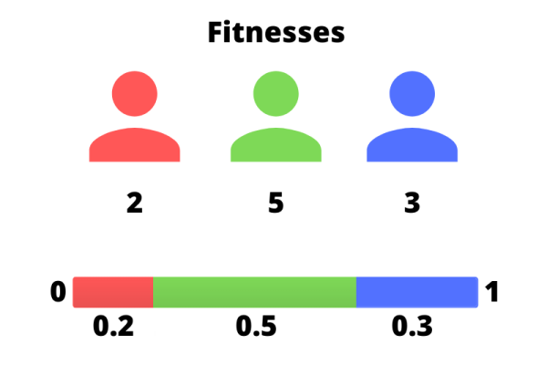
Fitness scores are then normalized so that they all add to one and can be placed along a segment of accumulated normalized fitnesses which runs from 0 to 1. The idea is that by sampling over this segment, individuals will be selected proportionally to their fitness score. Once again, this is only one method, called fitness proportionate selection, and many others exist.

// Evaluate population
const fitnesses = population.map(fitness);
const totalFitnesses = fitnesses.reduce((accumulator, currentValue) => accumulator + currentValue, 0);
const normalizedFitnesses = fitnesses.map(x => x / totalFitnesses);
const accumulatedNormalizedFitnesses = normalizedFitnesses.map(function (value) { return this.accumulator += value; }, { accumulator: 0 });

// Evaluate population

const fitnesses = population.map(fitness);

const totalFitnesses = fitnesses.reduce((accumulator, currentValue) => accumulator + currentValue, 0);

const normalizedFitnesses = fitnesses.map(x => x / totalFitnesses);

const accumulatedNormalizedFitnesses = normalizedFitnesses.map(function (value) { return this.accumulator += value; }, { accumulator: 0 });

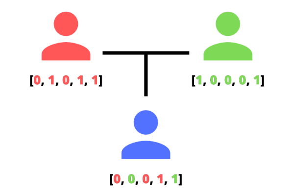
Once we are ready to sample from a distribution of better solutions, we can use the first genetic operator, crossover, to generate a new population from the previous one. As with most aspects of genetic algorithms, crossover comes in many forms, whether it is the number of parents, the way they are recombined to form children, and the number of children generated per crossover. Here, we will keep it simple with only two parents, a uniform recombination where each bit is randomly sampled from either parent with equal probability, and one child per pair. We will then repeat this process so as to obtain a new population of the same size as the previous one.

// Breed population
const newPopulation = [];

for (let i = 0; i < populationSize; i++) {
	const motherThreshold = Math.random();
	const mother = population[accumulatedNormalizedFitnesses.findIndex(x => x >= motherThreshold)];

	const fatherThreshold = Math.random();
	const father = population[accumulatedNormalizedFitnesses.findIndex(x => x >= fatherThreshold)];

	const child = Array.from({length: arraySize}, (value, index) => Math.random() > 0.5 ? mother[index] : father[index]);

	newPopulation.push(child);
}

// Replace parents with children
population = newPopulation;

// Breed population

const newPopulation = [];

for (let i = 0; i < populationSize; i++) {

const motherThreshold = Math.random();

const mother = population[accumulatedNormalizedFitnesses.findIndex(x => x >= motherThreshold)];

const fatherThreshold = Math.random();

const father = population[accumulatedNormalizedFitnesses.findIndex(x => x >= fatherThreshold)];

const child = Array.from({length: arraySize}, (value, index) => Math.random() > 0.5 ? mother[index] : father[index]);

newPopulation.push(child);

}

// Replace parents with children

population = newPopulation;

Now that a new population has replaced the previous one, it is time for a second genetic operator to come into play: mutation. At this stage, it won’t come as a surprise that mutation also exists in many shapes, though in the case of a bit array, it makes sense to simply flip each bit with a low probability. In our case, 0.1% seems to yield optimal results. Without mutation, the population is likely to converge towards a single local minimum, and the lack of diversity in the gene pool will render recombination useless. However, too high a mutation rate will hijack the population from its natural path, preventing the increase of its overall fitness.

// Configuration
const mutationRate = 0.001; // Mutation rate per bit

// ...

// Mutate population
population = population.map(individual => individual.map(value => Math.random() < mutationRate ? 1 - value : value));

// Configuration

const mutationRate = 0.001; // Mutation rate per bit

// ...

// Mutate population

population = population.map(individual => individual.map(value => Math.random() < mutationRate ? 1 - value : value));

And this is it for our algorithm! We can let it run for whatever amount of generations we like and add some logs to follow its progression:

console.log('Max fitness:');
console.log(Math.max(...fitnesses));

console.log('Average fitness:');
console.log(fitnesses.reduce((accumulator, currentValue) => accumulator + currentValue, 0) / fitnesses.length);

console.log('Max fitness:');

console.log(Math.max(...fitnesses));

console.log('Average fitness:');

console.log(fitnesses.reduce((accumulator, currentValue) => accumulator + currentValue, 0) / fitnesses.length);

I recommend playing with the parameters to see how they affect the performance of our algorithm, though it is important to note that in a way, the fitness function is one of them. For instance, I was able to get significantly better results by squaring the previous function, whose output ranged between zero and one, therefore penalizing lower scores compared to the higher ones in a nonlinear fashion.

const fitness = function(individual) {
	return (1 - individual
		.map((value, index) => Math.abs(value - solution[index]))
		.reduce((accumulator, currentValue) => accumulator + currentValue)
		/ arraySize) ** 2;
}

const fitness = function(individual) {

return (1 - individual

.map((value, index) => Math.abs(value - solution[index]))

.reduce((accumulator, currentValue) => accumulator + currentValue)

/ arraySize) ** 2;

}

One last example before we finish: we can use our algorithm to guess a mystery number. All we have to do is convert our bit array to its number representation, and base our fitness score on how different the representation is from the mystery number. $\frac{1}{1 + |r – m|}$ will yield values between 0 and 1, and despite working in a completely different fashion from bitwise comparison, our algorithm will guess our mystery number in no time!

const mystery = 801;

const fitness = function(individual) {
	let representation = 0;

	for (let i = 0; i < arraySize; i++) {
		representation += individual[i] * 2 ** i;
	}

	return 1 / (1 + Math.abs(representation - mystery));
}

const mystery = 801;

const fitness = function(individual) {

let representation = 0;

for (let i = 0; i < arraySize; i++) {

representation += individual[i] * 2 ** i;

}

return 1 / (1 + Math.abs(representation - mystery));

}

Collaborative filtering in PHP

In the era of PyTorch and TensorFlow 2.0, one may wonder why PHP would even come to mind when mentioning machine learning. No eager execution, no automatic differentiation, no vectorization of operations, no array broadcasting. It sounds hard to even think of implementing an algorithm without all these features and tools, let alone have it reach an acceptable level of performance.

And yet, PHP still dominates the world of web development. This is notably the case for e-commerce, where four of the top five players (WooCommerce, Magento, VirtueMart and PrestaShop), all written in PHP, already account for 45% of the worldwide market share. As online retail keeps growing (it now accounts for more than three-quarters of overall retail growth), it is also becoming more competitive, and retailers are on the look out for any possible way to boost their sales. Using a recommender system to highlight the products a customer is the most likely to buy is one of them.

While any large e-commerce player will have ample opportunity to build separate machine learning modules using an adequate framework, it is not the case for the majority of small retailers whose infrastructure is in no way designed to support anything other than the monolith that manages their entire business. What to do in such cases?

The idea is to keep it simple. We’ll be implementing the classic low-rank matrix factorization algorithm, using the best tools PHP has to offer. In this case, MathPHP will take care of all the linear algebra and statistics for us.

Let’s start by defining our data. We have users, and we have products. They can be linked together by what we’re going to call a score: there are many ways to build it, but most likely it will be either a rating (e.g. 1 to 5 stars) or a purchase indicator (1 if the user bought the product, 0 else). We’ll use $s(i, j)$ to denote the score given to product $i$ by user $j$, not necessarily defined for all pairs, and $S$ the set of pairs $(i, j)$ for which $s(i, j)$ is defined (i.e. a rating is available).

Now on to our model. The idea is to represent a product with $n$ features, and a user with $n$ weights, each expressing the correlation bewteen the score they would give a product and one of its the features. Therefore, a prediction of the score is given by the following:

$\sum\limits_{k = 1}^{n} u_k p_k$

Or, representing our users and products by vectors, simply $\vec{u} \cdot \vec{p}$. In order to minimize the difference between the predicted scores and the real ones, we will be working with the following cost function:

$J = \frac{1}{2} \sum\limits_{(i, j) \in S} (\vec{u_j} \cdot \vec{p_i} – s(i, j))^2 + \frac{\lambda}{2} \sum\limits_{i = 1}^{n_p} \|\vec{p_i}\|^2 + \frac{\lambda}{2} \sum\limits_{j = 1}^{n_u} \|\vec{u_j}\|^2$

The first term sums the squares of the differences between the predictions and the targets, while the other two are regularization terms ($L^2$ here but other methods can be used). This optimization objective yields the following gradients:

$\frac{\partial J}{\partial \vec{p_i}} = \sum\limits_{j \mid (i, j) \in S} (\vec{u_j} \cdot \vec{p_i} – s(i, j)) \vec{u_j} + \lambda \vec{p_i}$

$\frac{\partial J}{\partial \vec{u_j}} = \sum\limits_{i \mid (i, j) \in S} (\vec{u_j} \cdot \vec{p_i} – s(i, j)) \vec{p_i} + \lambda \vec{u_j}$

We can then update $\vec{p_i}$ and $\vec{u_j}$ using gradient descent, or one of its more advanced variations such as Adam. In the case of the former, which we’ll use for the sake of simplicity, this gives:

$\vec{p_i} := \vec{p_i} – \alpha \frac{\partial J}{\partial \vec{p_i}}$

$\vec{u_j} := \vec{u_j} – \alpha \frac{\partial J}{\partial \vec{u_j}}$

where $\alpha$ is the chosen learning rate.

How does this translate into code? Let’s suppose we have the following:

$products, a collection of Product objects
$users, a collection of Users objects
$ratings, a collection of Rating objects, with the product, user and rating properties

Let’s start by importing the required classes and setting up our configuration:

use MathPHP\LinearAlgebra\Vector;
use MathPHP\Probability\Distribution\Continuous\Normal;

// Configuration
$embeddingDimension = 8; // The number of dimensions we will represent our products (and users) with
$learningRate = 1e-3; // Our optimizer's learning rate
$lambda = 1e-1; // The regularization parameter
$distribution = new Normal(0, 1); // The distribution used to sample the initial values for our embeddings
$epochs = 500; // The number of epochs to train for

use MathPHP\LinearAlgebra\Vector;

use MathPHP\Probability\Distribution\Continuous\Normal;

// Configuration

$embeddingDimension = 8; // The number of dimensions we will represent our products (and users) with

$learningRate = 1e-3; // Our optimizer's learning rate

$lambda = 1e-1; // The regularization parameter

$distribution = new Normal(0, 1); // The distribution used to sample the initial values for our embeddings

$epochs = 500; // The number of epochs to train for

We’ll be using SplObjectStorage to store our embeddings, so that we don’t have to modify or extend our e-commerce software’s classes, using objects as keys instead. We will then initialize them using values from the chosen distribution (here a normal distribution of mean 0 and standard deviation 1, though other techniques can be used).

// Initialize object storage for embeddings
$embeddingStorage = new SplObjectStorage();

// Initialize product embeddings with random values
foreach ($products as $product) {
	$embeddingStorage[$product] = new Vector(array_map(function($value) use($distribution) {
		return $distribution->rand();
	}, range(0, $embeddingDimension - 1)));
}

// Initialize user embeddings with random values
foreach ($users as $user) {
	$embeddingStorage[$user] = new Vector(array_map(function($value) use($distribution) {
		return $distribution->rand();
	}, range(0, $embeddingDimension - 1)));
}

// Initialize object storage for embeddings

$embeddingStorage = new SplObjectStorage();

// Initialize product embeddings with random values

foreach ($products as $product) {

$embeddingStorage[$product] = new Vector(array_map(function($value) use($distribution) {

return $distribution->rand();

}, range(0, $embeddingDimension - 1)));

}

// Initialize user embeddings with random values

foreach ($users as $user) {

$embeddingStorage[$user] = new Vector(array_map(function($value) use($distribution) {

return $distribution->rand();

}, range(0, $embeddingDimension - 1)));

}

Now onto the first epoch. We’ll use the same method to store our gradients:

// Initialize object storage for gradients
$gradientStorage = new SplObjectStorage();

foreach ($products as $product) {
	$gradientStorage[$product] = new Vector(array_fill(0, $embeddingDimension, 0));
}

foreach ($users as $user) {
	$gradientStorage[$user] = new Vector(array_fill(0, $embeddingDimension, 0));
}

// Initialize object storage for gradients

$gradientStorage = new SplObjectStorage();

foreach ($products as $product) {

$gradientStorage[$product] = new Vector(array_fill(0, $embeddingDimension, 0));

}

foreach ($users as $user) {

$gradientStorage[$user] = new Vector(array_fill(0, $embeddingDimension, 0));

}

We can then loop through the ratings, and for each of them, compute the corresponding gradient part for the associated product and user. After this, we sum these gradient parts so as to obtain the full gradient in the above formula, minus the regularization terms.

// Loop through ratings to compute gradients
foreach ($ratings as $rating) {
	$gradientStorage[$rating->product] = $gradientStorage[$rating->product]->add($embeddingStorage[$rating->user]->scalarMultiply($embeddingStorage[$rating->user]->dotProduct($embeddingStorage[$rating->product]) - $rating->value));

	$gradientStorage[$rating->user] = $gradientStorage[$rating->user]->add($embeddingStorage[$rating->product]->scalarMultiply($embeddingStorage[$rating->user]->dotProduct($embeddingStorage[$rating->product]) - $rating->value));
}

// Loop through ratings to compute gradients

foreach ($ratings as $rating) {

$gradientStorage[$rating->product] = $gradientStorage[$rating->product]->add($embeddingStorage[$rating->user]->scalarMultiply($embeddingStorage[$rating->user]->dotProduct($embeddingStorage[$rating->product]) - $rating->value));

$gradientStorage[$rating->user] = $gradientStorage[$rating->user]->add($embeddingStorage[$rating->product]->scalarMultiply($embeddingStorage[$rating->user]->dotProduct($embeddingStorage[$rating->product]) - $rating->value));

}

Finally, we perform gradient descent, subtracting the gradients from the ratings as well as those from the regularization terms:

// Perform gradient descent
foreach ($products as $product) {
	$embeddingStorage[$product] = $embeddingStorage[$product]->subtract($gradientStorage[$product]->add($embeddingStorage[$product]->scalarMultiply($lambda))->scalarMultiply($learningRate));
}

foreach ($users as $user) {
	$embeddingStorage[$user] = $embeddingStorage[$user]->subtract($gradientStorage[$user]->add($embeddingStorage[$user]->scalarMultiply($lambda))->scalarMultiply($learningRate));
}

// Perform gradient descent

foreach ($products as $product) {

$embeddingStorage[$product] = $embeddingStorage[$product]->subtract($gradientStorage[$product]->add($embeddingStorage[$product]->scalarMultiply($lambda))->scalarMultiply($learningRate));

}

foreach ($users as $user) {

$embeddingStorage[$user] = $embeddingStorage[$user]->subtract($gradientStorage[$user]->add($embeddingStorage[$user]->scalarMultiply($lambda))->scalarMultiply($learningRate));

}

Now all there is left to do is wrap the code for the epoch in a loop and let it run for the specified number of times. Once this is done, obtaining a prediction is as simple as this:

$prediction = $embeddingStorage[$user]->dotProduct($embeddingStorage[$product]);

1	$prediction = $embeddingStorage[$user]->dotProduct($embeddingStorage[$product]);

It is also possible to look for similar products by comparing their embeddings:

$difference = $embeddingStorage[$product1]->subtract($embeddingStorage[$product2])->l2Norm();

1	$difference = $embeddingStorage[$product1]->subtract($embeddingStorage[$product2])->l2Norm();

You may have noticed that if a user hasn’t, say, rated or bought a product yet, the optimization objective will only be comprised of the regularization terms, leading to the user’s representation being a vector of zeros, and therefore predicting a score of zero for any product. This problem is often solved with mean normalization, which consists in subtracting, for each product, the mean of its ratings across all users before running the algorithm (and adding it back after prediction, of course).

However, all this will achieve in those cases is predict the average score instead of zero, and normalization over small samples may cause the model to be a lot less robust. For these reasons, I would suggest to simply ignore users and products under a certain threshold of ratings.

The full implementation is as follows:

use MathPHP\LinearAlgebra\Vector;
use MathPHP\Probability\Distribution\Continuous\Normal;

// Configuration
$embeddingDimension = 2; // The number of dimensions we will represent our products (and users) with
$learningRate = 1e-3; // Our optimizer's learning rate
$lambda = 1e-1; // The regularization parameter
$distribution = new Normal(0, 1); // The distribution used to sample the initial values for our embeddings
$epochs = 5000; // The number of epochs to train for

// Initialize object storage for embeddings
$embeddingStorage = new SplObjectStorage();

// Initialize product embeddings with random values
foreach ($products as $product) {
	$embeddingStorage[$product] = new Vector(array_map(function($value) use($distribution) {
		return $distribution->rand();
	}, range(0, $embeddingDimension - 1)));
}

// Initialize user embeddings with random values
foreach ($users as $user) {
	$embeddingStorage[$user] = new Vector(array_map(function($value) use($distribution) {
		return $distribution->rand();
	}, range(0, $embeddingDimension - 1)));
}

for ($i = 0; $i < $epochs; $i++) {
	// Initialize object storage for gradients
	$gradientStorage = new SplObjectStorage();

	foreach ($products as $product) {
		$gradientStorage[$product] = new Vector(array_fill(0, $embeddingDimension, 0));
	}

	foreach ($users as $user) {
		$gradientStorage[$user] = new Vector(array_fill(0, $embeddingDimension, 0));
	}
	
	// Loop through ratings to compute gradients
	foreach ($ratings as $rating) {
		$gradientStorage[$rating->product] = $gradientStorage[$rating->product]->add($embeddingStorage[$rating->user]->scalarMultiply($embeddingStorage[$rating->user]->dotProduct($embeddingStorage[$rating->product]) - $rating->value));

		$gradientStorage[$rating->user] = $gradientStorage[$rating->user]->add($embeddingStorage[$rating->product]->scalarMultiply($embeddingStorage[$rating->user]->dotProduct($embeddingStorage[$rating->product]) - $rating->value));
	}

	// Perform gradient descent
	foreach ($products as $product) {
		$embeddingStorage[$product] = $embeddingStorage[$product]->subtract($gradientStorage[$product]->add($embeddingStorage[$product]->scalarMultiply($lambda))->scalarMultiply($learningRate));
	}

	foreach ($users as $user) {
		$embeddingStorage[$user] = $embeddingStorage[$user]->subtract($gradientStorage[$user]->add($embeddingStorage[$user]->scalarMultiply($lambda))->scalarMultiply($learningRate));
	}
}

use MathPHP\LinearAlgebra\Vector;

use MathPHP\Probability\Distribution\Continuous\Normal;

// Configuration

$embeddingDimension = 2; // The number of dimensions we will represent our products (and users) with

$learningRate = 1e-3; // Our optimizer's learning rate

$lambda = 1e-1; // The regularization parameter

$distribution = new Normal(0, 1); // The distribution used to sample the initial values for our embeddings

$epochs = 5000; // The number of epochs to train for

// Initialize object storage for embeddings

$embeddingStorage = new SplObjectStorage();

// Initialize product embeddings with random values

foreach ($products as $product) {

$embeddingStorage[$product] = new Vector(array_map(function($value) use($distribution) {

return $distribution->rand();

}, range(0, $embeddingDimension - 1)));

}

// Initialize user embeddings with random values

foreach ($users as $user) {

$embeddingStorage[$user] = new Vector(array_map(function($value) use($distribution) {

return $distribution->rand();

}, range(0, $embeddingDimension - 1)));

}

for ($i = 0; $i < $epochs; $i++) {

// Initialize object storage for gradients

$gradientStorage = new SplObjectStorage();

foreach ($products as $product) {

$gradientStorage[$product] = new Vector(array_fill(0, $embeddingDimension, 0));

}

foreach ($users as $user) {

$gradientStorage[$user] = new Vector(array_fill(0, $embeddingDimension, 0));

}

// Loop through ratings to compute gradients

foreach ($ratings as $rating) {

}

// Perform gradient descent

foreach ($products as $product) {

$embeddingStorage[$product] = $embeddingStorage[$product]->subtract($gradientStorage[$product]->add($embeddingStorage[$product]->scalarMultiply($lambda))->scalarMultiply($learningRate));

}

foreach ($users as $user) {

$embeddingStorage[$user] = $embeddingStorage[$user]->subtract($gradientStorage[$user]->add($embeddingStorage[$user]->scalarMultiply($lambda))->scalarMultiply($learningRate));

}

And this is all you need to implement collaborative filtering on any of the e-commerce systems built with PHP.

Logistic regression and support vector machines

Logistic regression and support vector machines are widely used supervised learning models that give us a fast and efficient way of classifying new data based on a training set of classified, old data. While they appear similar, and often yield comparable results, they work in fundamentally different ways and both have their specificities.

Logistic regression, for a start, provides us with what we call a probabilistic model: applying that model to an unclassified entry yields the probability that it belongs to the class in question. In other terms: $h(\vec{x}) = \frac{1}{1 + e^{\large – \vec{\theta} \cdot \vec{x}}} = P(y = 1)$, where $h(\vec{x})$ is the hypothesis, $\vec{\theta}$ the computed parameters, $\vec{x}$ an entry and $y$ the actual classification (unknown) of that entry.

But then, in cases where a categorization is always required, it is common for engineers and data scientists to assign $\vec{x}$ to the class with the highest probability, even if it’s not very high, that is:

$y = \begin{cases} 1 & \text{if } h(\vec{x}) \geq \frac{1}{2} \\ 0 & \text{otherwise} \end{cases}$

As the logistic function is monotonically increasing, this correponds to:

$y = \begin{cases} 1 & \text{if } \vec{\theta} \cdot \vec{x} \geq 0 \\ 0 & \text{otherwise} \end{cases}$

This is, in fact, the exact hypothesis of a support vector machine (only with a different $\vec{\theta}$), which directly yields this deterministic prediction without going through the probability stage. It is, however, possible to obtain an equivalent probability using Platt scaling, which means that at this point, the two models are very similar.

In the end, the main difference between them lies in the way they are trained. Support vector machines are what we call a large margin classifier, and they work by finding the optimal separating hyperplane for the data they are provided: that is, the one that maximizes the distance from it to the nearest data point on each side.

This training is achieved through the minimization of different cost functions. For logistic regression, the cost function can be expressed as the following:

$\frac{1}{m} \sum\limits_{i = 1}^{m} (y_i (- \ln(\frac{1}{1 + e^{\large – \vec{\theta} \cdot \vec{x_i}}})) + (1 – y_i) (-\ln(1 – \frac{1}{1 + e^{\large – \vec{\theta} \cdot \vec{x_i}}})) + \frac{\lambda}{2} \|\vec{\theta}\|^2)$

(Note: the last term is used to prevent the model from overfitting, that is performing very well on the training set but failing to predict new entries. This technique is known as regularization, and can be adjusted with the parameter $\lambda$. We are using the $L^2$ norm here, but it is also possible to use the $L^1$ norm or a linear combination of both.)

The cost function above is in fact based on two sub-functions, one that is used if the entry is positive ($y = 1$), $– \ln(h(\vec{x}))$, and another if it is negative ($y = 0$), $-\ln(1 – h(\vec{x}))$. They are plotted below.

Support vector machines, on the other hand, are trained by minimizing the following cost function:

$\frac{1}{m} \sum\limits_{i = 1}^{m} (y_i \max(0, 1 – \vec{\theta} \cdot \vec{x_i}) + (1 – y_i) \max(0, 1 + \vec{\theta} \cdot \vec{x_i}) + \frac{\lambda}{2} \|\vec{\theta}\|^2)$

(Note: A different notation is traditionally used for support vector machines, but I’ll stick to this one for the sake of comparison.)

The two corresponding sub-functions are plotted below:

They are very similar to the ones used in logistic regression, except that they end more abruptly, placing no penalty on values of $\vec{\theta} \cdot \vec{x}$ greater than $1$ if $y = 1$, or smaller than $-1$ if $y = 0$. This clear delimitation allows support vector machines to separate data with as high a margin as possible. Note that with $\lambda$ very small (little to no regularization), this approach will be too sensitive to outliers and may not yield a truly optimal result.

But in the end, the most important difference beween logistic regression and support vector machines is how they work with kernels. Kernels are very useful when the data is not linearly separable: they allow us to map our entries ($\in \mathbb R^{n}$) to a new set of higher-dimensional entries ($\in \mathbb R ^{m}$) which can now be separated by an $m – 1$-dimensional hyperplane. A common example is the radial basis function kernel, which maps each entry in the data set to a decreasing function of the squared Euclidean distance between itself and each other entry: the associated kernel function is $K(\vec{x_1}, \vec{x_2}) = \exp\left(-\frac{\|\vec{x_1} – \vec{x_2}\|^2}{2\sigma^2}\right)$. A wide variety of kernels exist, from polynomial to string kernels (useful for text inputs).

Kernels can be used with pretty much every machine learning algorithm, but they are particularly efficient with support vector machines. This is because it’s possible to use sequential minimal optimization, an algorithm that partitions the training problem into smaller ones that can be solved analytically, in their implementation. This speeds up training significantly.

Now what about the implementation? Both logistic regression and SVMs are supported by MLlib. A simple logistic regression can be implemented as follows:

// Load training data
val training = spark.read.format("libsvm").load("data/mllib/sample_libsvm_data.txt")

val logisticRegression = new LogisticRegression()
    .setMaxIter(10)
    .setRegParam(0.3)
    .setElasticNetParam(0.8)

// Fit the model
val logisticRegressionModel = logisticRegression.fit(training)

// Print the coefficients and intercept for logistic regression
println(s"Coefficients: ${logisticRegressionModel.coefficients} Intercept: ${logisticRegressionModel.intercept}")

// Load training data

val training = spark.read.format("libsvm").load("data/mllib/sample_libsvm_data.txt")

val logisticRegression = new LogisticRegression()

.setMaxIter(10)

.setRegParam(0.3)

.setElasticNetParam(0.8)

// Fit the model

val logisticRegressionModel = logisticRegression.fit(training)

// Print the coefficients and intercept for logistic regression

println(s"Coefficients: ${logisticRegressionModel.coefficients} Intercept: ${logisticRegressionModel.intercept}")

(Note: setRegParam sets the regularization parameter $\lambda$, while setElasticNetParam sets the mix between the use of the $L^1$ and $L^2$ norms, from 0 for $L^2$ to 1 for $L^1$.)

And a support vector machine (with gradient descent) as the following:

// Load training data
val training = spark.read.format("libsvm").load("data/mllib/sample_libsvm_data.txt")

// Run training algorithm to build the model
val numIterations = 100
val svmModel = SVMWithSGD.train(training, numIterations)

// Print the weights and intercept for the support vector machine
println(s"Weights: ${svmModel.weights} Intercept: ${svmModel.intercept}")

// Load training data

val training = spark.read.format("libsvm").load("data/mllib/sample_libsvm_data.txt")

// Run training algorithm to build the model

val numIterations = 100

val svmModel = SVMWithSGD.train(training, numIterations)

// Print the weights and intercept for the support vector machine

println(s"Weights: ${svmModel.weights} Intercept: ${svmModel.intercept}")

What about kernels? Unfortunately, they’re not supported by MLlib just yet, but we can use TensorFlow:

# Radial basis function (Gaussian) kernel
gamma = tf.constant(-50.0)
dist = tf.reduce_sum(tf.square(x_data), 1)
dist = tf.reshape(dist, [-1,1])
sq_dists = tf.add(tf.subtract(dist, tf.multiply(2., tf.matmul(x_data, tf.transpose(x_data)))), tf.transpose(dist))
my_kernel = tf.exp(tf.multiply(gamma, tf.abs(sq_dists)))

# Compute SVM Model
first_term = tf.reduce_sum(b)
b_vec_cross = tf.matmul(tf.transpose(b), b)
y_target_cross = tf.matmul(y_target, tf.transpose(y_target))
second_term = tf.reduce_sum(tf.multiply(my_kernel, tf.multiply(b_vec_cross, y_target_cross)))
loss = tf.negative(tf.subtract(first_term, second_term))

# And then go on to handle prediction and training...
# ...

# Radial basis function (Gaussian) kernel

gamma = tf.constant(-50.0)

dist = tf.reduce_sum(tf.square(x_data), 1)

dist = tf.reshape(dist, [-1,1])

sq_dists = tf.add(tf.subtract(dist, tf.multiply(2., tf.matmul(x_data, tf.transpose(x_data)))), tf.transpose(dist))

my_kernel = tf.exp(tf.multiply(gamma, tf.abs(sq_dists)))

# Compute SVM Model

first_term = tf.reduce_sum(b)

b_vec_cross = tf.matmul(tf.transpose(b), b)

y_target_cross = tf.matmul(y_target, tf.transpose(y_target))

second_term = tf.reduce_sum(tf.multiply(my_kernel, tf.multiply(b_vec_cross, y_target_cross)))

loss = tf.negative(tf.subtract(first_term, second_term))

# And then go on to handle prediction and training...

# ...

And this is it for now. Knowing which algorithm to choose is indubitably helpful, but it is important to keep in mind that in many cases, the quality and quantity of the training set as well as the parametrization of the model matter more than the choice of the algorithm itself.