Genetic algorithms are a subclass of evolutionary algorithms which are inspired by the mechanism of natural selection. Mainly used for complex optimization and search problems, they consist in letting a population of potential solutions evolve through selection of the fittest, reproduction and mutation.
The first step consists in generating an initial population, usually at random, though any knowledge of the distribution of optimal solutions may be used to sample from specific regions of the search space. Bit arrays are a standard representation for candidates, and in this example we will conveniently use arrays of ones and zeros of size arraySize, and generate populationSize of them:
|
1 2 3 4 5 6 7 8 9 10 11 12 |
// Configuration const populationSize = 100; // Size of the population const arraySize = 100; // Size of a candidate in bits // ... // Initialize population let population = []; for (let i = 0; i < populationSize; i++) { population.push(Array.from({length: arraySize}, () => Math.round(Math.random()));); } |
The cornerstone of our algorithm will be to repeatedly rate our population. This is achieved by defining a fitness function, which will be a measure of how good a candidate is. Since this is a theoretical example and we have no practical application for our bit arrays, we will simply define a hard-coded solution and measure a candidate by how much it differs from that target, bitwise:
|
1 2 3 4 5 6 7 8 |
const solution = [0, 1, 1, 1, 1, 1, 0, 1, 1, 1, 0, 1, 1, 1, 1, 1, 0, 1, 1, 0, 1, 1, 1, 1, 1, 1, 0, 1, 1, 0, 0, 1, 1, 1, 1, 1, 0, 1, 1, 0, 0, 1, 1, 1, 1, 1, 0, 1, 1, 0, 0, 1, 1, 0, 1, 0, 0, 1, 1, 0, 0, 1, 1, 1, 1, 1, 0, 1, 1, 0, 0, 1, 1, 1, 1, 1, 0, 1, 1, 0, 0, 1, 1, 1, 0, 1, 0, 1, 1, 0, 0, 1, 1, 1, 0, 1, 0, 1, 1, 0]; const fitness = function(individual) { return 1 - individual .map((value, index) => Math.abs(value - solution[index])) .reduce((accumulator, currentValue) => accumulator + currentValue, 0) / arraySize; } |
Now our initial population has been generated, we can begin the cycle of selection, reproduction and mutation. We will go through fixed number of iterations (generations), however it is possible to stop the algorithm when it finds a solution that satisfies a required fitness threshold, or when generations stop improving and additional cycles bring no value.
|
1 2 3 4 5 6 7 8 9 |
// Configuration const generations = 1000; // Number of generations // ... // Main loop for (let generation = 0; generation < generations; generation++) { // ... } |
First, we evaluate our population by computing the fitness of each individual. Variants are used where only a fraction of the population is evaluated so as to minimize computational cost.
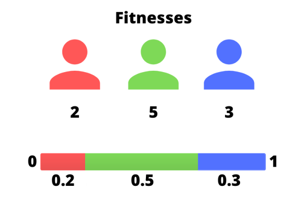
Fitness scores are then normalized so that they all add to one and can be placed along a segment of accumulated normalized fitnesses which runs from 0 to 1. The idea is that by sampling over this segment, individuals will be selected proportionally to their fitness score. Once again, this is only one method, called fitness proportionate selection, and many others exist.

|
1 2 3 4 5 |
// Evaluate population const fitnesses = population.map(fitness); const totalFitnesses = fitnesses.reduce((accumulator, currentValue) => accumulator + currentValue, 0); const normalizedFitnesses = fitnesses.map(x => x / totalFitnesses); const accumulatedNormalizedFitnesses = normalizedFitnesses.map(function (value) { return this.accumulator += value; }, { accumulator: 0 }); |
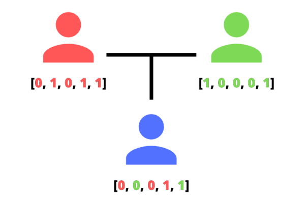
Once we are ready to sample from a distribution of better solutions, we can use the first genetic operator, crossover, to generate a new population from the previous one. As with most aspects of genetic algorithms, crossover comes in many forms, whether it is the number of parents, the way they are recombined to form children, and the number of children generated per crossover. Here, we will keep it simple with only two parents, a uniform recombination where each bit is randomly sampled from either parent with equal probability, and one child per pair. We will then repeat this process so as to obtain a new population of the same size as the previous one.

|
1 2 3 4 5 6 7 8 9 10 11 12 13 14 15 16 17 |
// Breed population const newPopulation = []; for (let i = 0; i < populationSize; i++) { const motherThreshold = Math.random(); const mother = population[accumulatedNormalizedFitnesses.findIndex(x => x >= motherThreshold)]; const fatherThreshold = Math.random(); const father = population[accumulatedNormalizedFitnesses.findIndex(x => x >= fatherThreshold)]; const child = Array.from({length: arraySize}, (value, index) => Math.random() > 0.5 ? mother[index] : father[index]); newPopulation.push(child); } // Replace parents with children population = newPopulation; |
Now that a new population has replaced the previous one, it is time for a second genetic operator to come into play: mutation. At this stage, it won’t come as a surprise that mutation also exists in many shapes, though in the case of a bit array, it makes sense to simply flip each bit with a low probability. In our case, 0.1% seems to yield optimal results. Without mutation, the population is likely to converge towards a single local minimum, and the lack of diversity in the gene pool will render recombination useless. However, too high a mutation rate will hijack the population from its natural path, preventing the increase of its overall fitness.
|
1 2 3 4 5 6 7 |
// Configuration const mutationRate = 0.001; // Mutation rate per bit // ... // Mutate population population = population.map(individual => individual.map(value => Math.random() < mutationRate ? 1 - value : value)); |
And this is it for our algorithm! We can let it run for whatever amount of generations we like and add some logs to follow its progression:
|
1 2 3 4 5 |
console.log('Max fitness:'); console.log(Math.max(...fitnesses)); console.log('Average fitness:'); console.log(fitnesses.reduce((accumulator, currentValue) => accumulator + currentValue, 0) / fitnesses.length); |
I recommend playing with the parameters to see how they affect the performance of our algorithm, though it is important to note that in a way, the fitness function is one of them. For instance, I was able to get significantly better results by squaring the previous function, whose output ranged between zero and one, therefore penalizing lower scores compared to the higher ones in a nonlinear fashion.
|
1 2 3 4 5 6 |
const fitness = function(individual) { return (1 - individual .map((value, index) => Math.abs(value - solution[index])) .reduce((accumulator, currentValue) => accumulator + currentValue) / arraySize) ** 2; } |
One last example before we finish: we can use our algorithm to guess a mystery number. All we have to do is convert our bit array to its number representation, and base our fitness score on how different the representation is from the mystery number. \(\frac{1}{1 + |r – m|}\) will yield values between 0 and 1, and despite working in a completely different fashion from bitwise comparison, our algorithm will guess our mystery number in no time!
|
1 2 3 4 5 6 7 8 9 10 11 |
const mystery = 801; const fitness = function(individual) { let representation = 0; for (let i = 0; i < arraySize; i++) { representation += individual[i] * 2 ** i; } return 1 / (1 + Math.abs(representation - mystery)); } |