Pierre-Henry Baudin – Software Engineer • Paris

An introduction to genetic algorithms

Genetic algorithms are a subclass of evolutionary algorithms which are inspired by the mechanism of natural selection. Mainly used for complex optimization and search problems, they consist in letting a population of potential solutions evolve through selection of the fittest, reproduction and mutation.

The first step consists in generating an initial population, usually at random, though any knowledge of the distribution of optimal solutions may be used to sample from specific regions of the search space. Bit arrays are a standard representation for candidates, and in this example we will conveniently use arrays of ones and zeros of size arraySize, and generate populationSize of them:

// Configuration
const populationSize = 100; // Size of the population
const arraySize = 100; // Size of a candidate in bits

// ...

// Initialize population
let population = [];

for (let i = 0; i < populationSize; i++) {
	population.push(Array.from({length: arraySize}, () => Math.round(Math.random())););
}

// Configuration

const populationSize = 100; // Size of the population

const arraySize = 100; // Size of a candidate in bits

// ...

// Initialize population

let population = [];

for (let i = 0; i < populationSize; i++) {

population.push(Array.from({length: arraySize}, () => Math.round(Math.random())););

}

The cornerstone of our algorithm will be to repeatedly rate our population. This is achieved by defining a fitness function, which will be a measure of how good a candidate is. Since this is a theoretical example and we have no practical application for our bit arrays, we will simply define a hard-coded solution and measure a candidate by how much it differs from that target, bitwise:

const solution = [0, 1, 1, 1, 1, 1, 0, 1, 1, 1, 0, 1, 1, 1, 1, 1, 0, 1, 1, 0, 1, 1, 1, 1, 1, 1, 0, 1, 1, 0, 0, 1, 1, 1, 1, 1, 0, 1, 1, 0, 0, 1, 1, 1, 1, 1, 0, 1, 1, 0, 0, 1, 1, 0, 1, 0, 0, 1, 1, 0, 0, 1, 1, 1, 1, 1, 0, 1, 1, 0, 0, 1, 1, 1, 1, 1, 0, 1, 1, 0, 0, 1, 1, 1, 0, 1, 0, 1, 1, 0, 0, 1, 1, 1, 0, 1, 0, 1, 1, 0];

const fitness = function(individual) {
	return 1 - individual
		.map((value, index) => Math.abs(value - solution[index]))
		.reduce((accumulator, currentValue) => accumulator + currentValue, 0)
		/ arraySize;
}

const solution = [0, 1, 1, 1, 1, 1, 0, 1, 1, 1, 0, 1, 1, 1, 1, 1, 0, 1, 1, 0, 1, 1, 1, 1, 1, 1, 0, 1, 1, 0, 0, 1, 1, 1, 1, 1, 0, 1, 1, 0, 0, 1, 1, 1, 1, 1, 0, 1, 1, 0, 0, 1, 1, 0, 1, 0, 0, 1, 1, 0, 0, 1, 1, 1, 1, 1, 0, 1, 1, 0, 0, 1, 1, 1, 1, 1, 0, 1, 1, 0, 0, 1, 1, 1, 0, 1, 0, 1, 1, 0, 0, 1, 1, 1, 0, 1, 0, 1, 1, 0];

const fitness = function(individual) {

return 1 - individual

.map((value, index) => Math.abs(value - solution[index]))

.reduce((accumulator, currentValue) => accumulator + currentValue, 0)

/ arraySize;

}

Now our initial population has been generated, we can begin the cycle of selection, reproduction and mutation. We will go through fixed number of iterations (generations), however it is possible to stop the algorithm when it finds a solution that satisfies a required fitness threshold, or when generations stop improving and additional cycles bring no value.

// Configuration
const generations = 1000; // Number of generations

// ...

// Main loop
for (let generation = 0; generation < generations; generation++) {
	// ...
}

// Configuration

const generations = 1000; // Number of generations

// ...

// Main loop

for (let generation = 0; generation < generations; generation++) {

// ...

}

First, we evaluate our population by computing the fitness of each individual. Variants are used where only a fraction of the population is evaluated so as to minimize computational cost.

Fitness scores are then normalized so that they all add to one and can be placed along a segment of accumulated normalized fitnesses which runs from 0 to 1. The idea is that by sampling over this segment, individuals will be selected proportionally to their fitness score. Once again, this is only one method, called fitness proportionate selection, and many others exist.

// Evaluate population
const fitnesses = population.map(fitness);
const totalFitnesses = fitnesses.reduce((accumulator, currentValue) => accumulator + currentValue, 0);
const normalizedFitnesses = fitnesses.map(x => x / totalFitnesses);
const accumulatedNormalizedFitnesses = normalizedFitnesses.map(function (value) { return this.accumulator += value; }, { accumulator: 0 });

// Evaluate population

const fitnesses = population.map(fitness);

const totalFitnesses = fitnesses.reduce((accumulator, currentValue) => accumulator + currentValue, 0);

const normalizedFitnesses = fitnesses.map(x => x / totalFitnesses);

const accumulatedNormalizedFitnesses = normalizedFitnesses.map(function (value) { return this.accumulator += value; }, { accumulator: 0 });

Once we are ready to sample from a distribution of better solutions, we can use the first genetic operator, crossover, to generate a new population from the previous one. As with most aspects of genetic algorithms, crossover comes in many forms, whether it is the number of parents, the way they are recombined to form children, and the number of children generated per crossover. Here, we will keep it simple with only two parents, a uniform recombination where each bit is randomly sampled from either parent with equal probability, and one child per pair. We will then repeat this process so as to obtain a new population of the same size as the previous one.

// Breed population
const newPopulation = [];

for (let i = 0; i < populationSize; i++) {
	const motherThreshold = Math.random();
	const mother = population[accumulatedNormalizedFitnesses.findIndex(x => x >= motherThreshold)];

	const fatherThreshold = Math.random();
	const father = population[accumulatedNormalizedFitnesses.findIndex(x => x >= fatherThreshold)];

	const child = Array.from({length: arraySize}, (value, index) => Math.random() > 0.5 ? mother[index] : father[index]);

	newPopulation.push(child);
}

// Replace parents with children
population = newPopulation;

// Breed population

const newPopulation = [];

for (let i = 0; i < populationSize; i++) {

const motherThreshold = Math.random();

const mother = population[accumulatedNormalizedFitnesses.findIndex(x => x >= motherThreshold)];

const fatherThreshold = Math.random();

const father = population[accumulatedNormalizedFitnesses.findIndex(x => x >= fatherThreshold)];

const child = Array.from({length: arraySize}, (value, index) => Math.random() > 0.5 ? mother[index] : father[index]);

newPopulation.push(child);

}

// Replace parents with children

population = newPopulation;

Now that a new population has replaced the previous one, it is time for a second genetic operator to come into play: mutation. At this stage, it won’t come as a surprise that mutation also exists in many shapes, though in the case of a bit array, it makes sense to simply flip each bit with a low probability. In our case, 0.1% seems to yield optimal results. Without mutation, the population is likely to converge towards a single local minimum, and the lack of diversity in the gene pool will render recombination useless. However, too high a mutation rate will hijack the population from its natural path, preventing the increase of its overall fitness.

// Configuration
const mutationRate = 0.001; // Mutation rate per bit

// ...

// Mutate population
population = population.map(individual => individual.map(value => Math.random() < mutationRate ? 1 - value : value));

// Configuration

const mutationRate = 0.001; // Mutation rate per bit

// ...

// Mutate population

population = population.map(individual => individual.map(value => Math.random() < mutationRate ? 1 - value : value));

And this is it for our algorithm! We can let it run for whatever amount of generations we like and add some logs to follow its progression:

console.log('Max fitness:');
console.log(Math.max(...fitnesses));

console.log('Average fitness:');
console.log(fitnesses.reduce((accumulator, currentValue) => accumulator + currentValue, 0) / fitnesses.length);

console.log('Max fitness:');

console.log(Math.max(...fitnesses));

console.log('Average fitness:');

console.log(fitnesses.reduce((accumulator, currentValue) => accumulator + currentValue, 0) / fitnesses.length);

I recommend playing with the parameters to see how they affect the performance of our algorithm, though it is important to note that in a way, the fitness function is one of them. For instance, I was able to get significantly better results by squaring the previous function, whose output ranged between zero and one, therefore penalizing lower scores compared to the higher ones in a nonlinear fashion.

const fitness = function(individual) {
	return (1 - individual
		.map((value, index) => Math.abs(value - solution[index]))
		.reduce((accumulator, currentValue) => accumulator + currentValue)
		/ arraySize) ** 2;
}

const fitness = function(individual) {

return (1 - individual

.map((value, index) => Math.abs(value - solution[index]))

.reduce((accumulator, currentValue) => accumulator + currentValue)

/ arraySize) ** 2;

}

One last example before we finish: we can use our algorithm to guess a mystery number. All we have to do is convert our bit array to its number representation, and base our fitness score on how different the representation is from the mystery number. $\frac{1}{1 + |r – m|}$ will yield values between 0 and 1, and despite working in a completely different fashion from bitwise comparison, our algorithm will guess our mystery number in no time!

const mystery = 801;

const fitness = function(individual) {
	let representation = 0;

	for (let i = 0; i < arraySize; i++) {
		representation += individual[i] * 2 ** i;
	}

	return 1 / (1 + Math.abs(representation - mystery));
}

const mystery = 801;

const fitness = function(individual) {

let representation = 0;

for (let i = 0; i < arraySize; i++) {

representation += individual[i] * 2 ** i;

}

return 1 / (1 + Math.abs(representation - mystery));

}

Collaborative filtering in PHP

In the era of PyTorch and TensorFlow 2.0, one may wonder why PHP would even come to mind when mentioning machine learning. No eager execution, no automatic differentiation, no vectorization of operations, no array broadcasting. It sounds hard to even think of implementing an algorithm without all these features and tools, let alone have it reach an acceptable level of performance.

And yet, PHP still dominates the world of web development. This is notably the case for e-commerce, where four of the top five players (WooCommerce, Magento, VirtueMart and PrestaShop), all written in PHP, already account for 45% of the worldwide market share. As online retail keeps growing (it now accounts for more than three-quarters of overall retail growth), it is also becoming more competitive, and retailers are on the look out for any possible way to boost their sales. Using a recommender system to highlight the products a customer is the most likely to buy is one of them.

While any large e-commerce player will have ample opportunity to build separate machine learning modules using an adequate framework, it is not the case for the majority of small retailers whose infrastructure is in no way designed to support anything other than the monolith that manages their entire business. What to do in such cases?

The idea is to keep it simple. We’ll be implementing the classic low-rank matrix factorization algorithm, using the best tools PHP has to offer. In this case, MathPHP will take care of all the linear algebra and statistics for us.

Let’s start by defining our data. We have users, and we have products. They can be linked together by what we’re going to call a score: there are many ways to build it, but most likely it will be either a rating (e.g. 1 to 5 stars) or a purchase indicator (1 if the user bought the product, 0 else). We’ll use $s(i, j)$ to denote the score given to product $i$ by user $j$, not necessarily defined for all pairs, and $S$ the set of pairs $(i, j)$ for which $s(i, j)$ is defined (i.e. a rating is available).

Now on to our model. The idea is to represent a product with $n$ features, and a user with $n$ weights, each expressing the correlation bewteen the score they would give a product and one of its the features. Therefore, a prediction of the score is given by the following:

$\sum\limits_{k = 1}^{n} u_k p_k$

Or, representing our users and products by vectors, simply $\vec{u} \cdot \vec{p}$. In order to minimize the difference between the predicted scores and the real ones, we will be working with the following cost function:

$J = \frac{1}{2} \sum\limits_{(i, j) \in S} (\vec{u_j} \cdot \vec{p_i} – s(i, j))^2 + \frac{\lambda}{2} \sum\limits_{i = 1}^{n_p} \|\vec{p_i}\|^2 + \frac{\lambda}{2} \sum\limits_{j = 1}^{n_u} \|\vec{u_j}\|^2$

The first term sums the squares of the differences between the predictions and the targets, while the other two are regularization terms ($L^2$ here but other methods can be used). This optimization objective yields the following gradients:

$\frac{\partial J}{\partial \vec{p_i}} = \sum\limits_{j \mid (i, j) \in S} (\vec{u_j} \cdot \vec{p_i} – s(i, j)) \vec{u_j} + \lambda \vec{p_i}$

$\frac{\partial J}{\partial \vec{u_j}} = \sum\limits_{i \mid (i, j) \in S} (\vec{u_j} \cdot \vec{p_i} – s(i, j)) \vec{p_i} + \lambda \vec{u_j}$

We can then update $\vec{p_i}$ and $\vec{u_j}$ using gradient descent, or one of its more advanced variations such as Adam. In the case of the former, which we’ll use for the sake of simplicity, this gives:

$\vec{p_i} := \vec{p_i} – \alpha \frac{\partial J}{\partial \vec{p_i}}$

$\vec{u_j} := \vec{u_j} – \alpha \frac{\partial J}{\partial \vec{u_j}}$

where $\alpha$ is the chosen learning rate.

How does this translate into code? Let’s suppose we have the following:

$products, a collection of Product objects
$users, a collection of Users objects
$ratings, a collection of Rating objects, with the product, user and rating properties

Let’s start by importing the required classes and setting up our configuration:

use MathPHP\LinearAlgebra\Vector;
use MathPHP\Probability\Distribution\Continuous\Normal;

// Configuration
$embeddingDimension = 8; // The number of dimensions we will represent our products (and users) with
$learningRate = 1e-3; // Our optimizer's learning rate
$lambda = 1e-1; // The regularization parameter
$distribution = new Normal(0, 1); // The distribution used to sample the initial values for our embeddings
$epochs = 500; // The number of epochs to train for

use MathPHP\LinearAlgebra\Vector;

use MathPHP\Probability\Distribution\Continuous\Normal;

// Configuration

$embeddingDimension = 8; // The number of dimensions we will represent our products (and users) with

$learningRate = 1e-3; // Our optimizer's learning rate

$lambda = 1e-1; // The regularization parameter

$distribution = new Normal(0, 1); // The distribution used to sample the initial values for our embeddings

$epochs = 500; // The number of epochs to train for

We’ll be using SplObjectStorage to store our embeddings, so that we don’t have to modify or extend our e-commerce software’s classes, using objects as keys instead. We will then initialize them using values from the chosen distribution (here a normal distribution of mean 0 and standard deviation 1, though other techniques can be used).

// Initialize object storage for embeddings
$embeddingStorage = new SplObjectStorage();

// Initialize product embeddings with random values
foreach ($products as $product) {
	$embeddingStorage[$product] = new Vector(array_map(function($value) use($distribution) {
		return $distribution->rand();
	}, range(0, $embeddingDimension - 1)));
}

// Initialize user embeddings with random values
foreach ($users as $user) {
	$embeddingStorage[$user] = new Vector(array_map(function($value) use($distribution) {
		return $distribution->rand();
	}, range(0, $embeddingDimension - 1)));
}

// Initialize object storage for embeddings

$embeddingStorage = new SplObjectStorage();

// Initialize product embeddings with random values

foreach ($products as $product) {

$embeddingStorage[$product] = new Vector(array_map(function($value) use($distribution) {

return $distribution->rand();

}, range(0, $embeddingDimension - 1)));

}

// Initialize user embeddings with random values

foreach ($users as $user) {

$embeddingStorage[$user] = new Vector(array_map(function($value) use($distribution) {

return $distribution->rand();

}, range(0, $embeddingDimension - 1)));

}

Now onto the first epoch. We’ll use the same method to store our gradients:

// Initialize object storage for gradients
$gradientStorage = new SplObjectStorage();

foreach ($products as $product) {
	$gradientStorage[$product] = new Vector(array_fill(0, $embeddingDimension, 0));
}

foreach ($users as $user) {
	$gradientStorage[$user] = new Vector(array_fill(0, $embeddingDimension, 0));
}

// Initialize object storage for gradients

$gradientStorage = new SplObjectStorage();

foreach ($products as $product) {

$gradientStorage[$product] = new Vector(array_fill(0, $embeddingDimension, 0));

}

foreach ($users as $user) {

$gradientStorage[$user] = new Vector(array_fill(0, $embeddingDimension, 0));

}

We can then loop through the ratings, and for each of them, compute the corresponding gradient part for the associated product and user. After this, we sum these gradient parts so as to obtain the full gradient in the above formula, minus the regularization terms.

// Loop through ratings to compute gradients
foreach ($ratings as $rating) {
	$gradientStorage[$rating->product] = $gradientStorage[$rating->product]->add($embeddingStorage[$rating->user]->scalarMultiply($embeddingStorage[$rating->user]->dotProduct($embeddingStorage[$rating->product]) - $rating->value));

	$gradientStorage[$rating->user] = $gradientStorage[$rating->user]->add($embeddingStorage[$rating->product]->scalarMultiply($embeddingStorage[$rating->user]->dotProduct($embeddingStorage[$rating->product]) - $rating->value));
}

// Loop through ratings to compute gradients

foreach ($ratings as $rating) {

$gradientStorage[$rating->product] = $gradientStorage[$rating->product]->add($embeddingStorage[$rating->user]->scalarMultiply($embeddingStorage[$rating->user]->dotProduct($embeddingStorage[$rating->product]) - $rating->value));

$gradientStorage[$rating->user] = $gradientStorage[$rating->user]->add($embeddingStorage[$rating->product]->scalarMultiply($embeddingStorage[$rating->user]->dotProduct($embeddingStorage[$rating->product]) - $rating->value));

}

Finally, we perform gradient descent, subtracting the gradients from the ratings as well as those from the regularization terms:

// Perform gradient descent
foreach ($products as $product) {
	$embeddingStorage[$product] = $embeddingStorage[$product]->subtract($gradientStorage[$product]->add($embeddingStorage[$product]->scalarMultiply($lambda))->scalarMultiply($learningRate));
}

foreach ($users as $user) {
	$embeddingStorage[$user] = $embeddingStorage[$user]->subtract($gradientStorage[$user]->add($embeddingStorage[$user]->scalarMultiply($lambda))->scalarMultiply($learningRate));
}

// Perform gradient descent

foreach ($products as $product) {

$embeddingStorage[$product] = $embeddingStorage[$product]->subtract($gradientStorage[$product]->add($embeddingStorage[$product]->scalarMultiply($lambda))->scalarMultiply($learningRate));

}

foreach ($users as $user) {

$embeddingStorage[$user] = $embeddingStorage[$user]->subtract($gradientStorage[$user]->add($embeddingStorage[$user]->scalarMultiply($lambda))->scalarMultiply($learningRate));

}

Now all there is left to do is wrap the code for the epoch in a loop and let it run for the specified number of times. Once this is done, obtaining a prediction is as simple as this:

$prediction = $embeddingStorage[$user]->dotProduct($embeddingStorage[$product]);

1	$prediction = $embeddingStorage[$user]->dotProduct($embeddingStorage[$product]);

It is also possible to look for similar products by comparing their embeddings:

$difference = $embeddingStorage[$product1]->subtract($embeddingStorage[$product2])->l2Norm();

1	$difference = $embeddingStorage[$product1]->subtract($embeddingStorage[$product2])->l2Norm();

You may have noticed that if a user hasn’t, say, rated or bought a product yet, the optimization objective will only be comprised of the regularization terms, leading to the user’s representation being a vector of zeros, and therefore predicting a score of zero for any product. This problem is often solved with mean normalization, which consists in subtracting, for each product, the mean of its ratings across all users before running the algorithm (and adding it back after prediction, of course).

However, all this will achieve in those cases is predict the average score instead of zero, and normalization over small samples may cause the model to be a lot less robust. For these reasons, I would suggest to simply ignore users and products under a certain threshold of ratings.

The full implementation is as follows:

use MathPHP\LinearAlgebra\Vector;
use MathPHP\Probability\Distribution\Continuous\Normal;

// Configuration
$embeddingDimension = 2; // The number of dimensions we will represent our products (and users) with
$learningRate = 1e-3; // Our optimizer's learning rate
$lambda = 1e-1; // The regularization parameter
$distribution = new Normal(0, 1); // The distribution used to sample the initial values for our embeddings
$epochs = 5000; // The number of epochs to train for

// Initialize object storage for embeddings
$embeddingStorage = new SplObjectStorage();

// Initialize product embeddings with random values
foreach ($products as $product) {
	$embeddingStorage[$product] = new Vector(array_map(function($value) use($distribution) {
		return $distribution->rand();
	}, range(0, $embeddingDimension - 1)));
}

// Initialize user embeddings with random values
foreach ($users as $user) {
	$embeddingStorage[$user] = new Vector(array_map(function($value) use($distribution) {
		return $distribution->rand();
	}, range(0, $embeddingDimension - 1)));
}

for ($i = 0; $i < $epochs; $i++) {
	// Initialize object storage for gradients
	$gradientStorage = new SplObjectStorage();

	foreach ($products as $product) {
		$gradientStorage[$product] = new Vector(array_fill(0, $embeddingDimension, 0));
	}

	foreach ($users as $user) {
		$gradientStorage[$user] = new Vector(array_fill(0, $embeddingDimension, 0));
	}
	
	// Loop through ratings to compute gradients
	foreach ($ratings as $rating) {
		$gradientStorage[$rating->product] = $gradientStorage[$rating->product]->add($embeddingStorage[$rating->user]->scalarMultiply($embeddingStorage[$rating->user]->dotProduct($embeddingStorage[$rating->product]) - $rating->value));

		$gradientStorage[$rating->user] = $gradientStorage[$rating->user]->add($embeddingStorage[$rating->product]->scalarMultiply($embeddingStorage[$rating->user]->dotProduct($embeddingStorage[$rating->product]) - $rating->value));
	}

	// Perform gradient descent
	foreach ($products as $product) {
		$embeddingStorage[$product] = $embeddingStorage[$product]->subtract($gradientStorage[$product]->add($embeddingStorage[$product]->scalarMultiply($lambda))->scalarMultiply($learningRate));
	}

	foreach ($users as $user) {
		$embeddingStorage[$user] = $embeddingStorage[$user]->subtract($gradientStorage[$user]->add($embeddingStorage[$user]->scalarMultiply($lambda))->scalarMultiply($learningRate));
	}
}

use MathPHP\LinearAlgebra\Vector;

use MathPHP\Probability\Distribution\Continuous\Normal;

// Configuration

$embeddingDimension = 2; // The number of dimensions we will represent our products (and users) with

$learningRate = 1e-3; // Our optimizer's learning rate

$lambda = 1e-1; // The regularization parameter

$distribution = new Normal(0, 1); // The distribution used to sample the initial values for our embeddings

$epochs = 5000; // The number of epochs to train for

// Initialize object storage for embeddings

$embeddingStorage = new SplObjectStorage();

// Initialize product embeddings with random values

foreach ($products as $product) {

$embeddingStorage[$product] = new Vector(array_map(function($value) use($distribution) {

return $distribution->rand();

}, range(0, $embeddingDimension - 1)));

}

// Initialize user embeddings with random values

foreach ($users as $user) {

$embeddingStorage[$user] = new Vector(array_map(function($value) use($distribution) {

return $distribution->rand();

}, range(0, $embeddingDimension - 1)));

}

for ($i = 0; $i < $epochs; $i++) {

// Initialize object storage for gradients

$gradientStorage = new SplObjectStorage();

foreach ($products as $product) {

$gradientStorage[$product] = new Vector(array_fill(0, $embeddingDimension, 0));

}

foreach ($users as $user) {

$gradientStorage[$user] = new Vector(array_fill(0, $embeddingDimension, 0));

}

// Loop through ratings to compute gradients

foreach ($ratings as $rating) {

}

// Perform gradient descent

foreach ($products as $product) {

$embeddingStorage[$product] = $embeddingStorage[$product]->subtract($gradientStorage[$product]->add($embeddingStorage[$product]->scalarMultiply($lambda))->scalarMultiply($learningRate));

}

foreach ($users as $user) {

$embeddingStorage[$user] = $embeddingStorage[$user]->subtract($gradientStorage[$user]->add($embeddingStorage[$user]->scalarMultiply($lambda))->scalarMultiply($learningRate));

}

And this is all you need to implement collaborative filtering on any of the e-commerce systems built with PHP.

Logistic regression and support vector machines

Logistic regression and support vector machines are widely used supervised learning models that give us a fast and efficient way of classifying new data based on a training set of classified, old data. While they appear similar, and often yield comparable results, they work in fundamentally different ways and both have their specificities.

Logistic regression, for a start, provides us with what we call a probabilistic model: applying that model to an unclassified entry yields the probability that it belongs to the class in question. In other terms: $h(\vec{x}) = \frac{1}{1 + e^{\large – \vec{\theta} \cdot \vec{x}}} = P(y = 1)$, where $h(\vec{x})$ is the hypothesis, $\vec{\theta}$ the computed parameters, $\vec{x}$ an entry and $y$ the actual classification (unknown) of that entry.

But then, in cases where a categorization is always required, it is common for engineers and data scientists to assign $\vec{x}$ to the class with the highest probability, even if it’s not very high, that is:

$y = \begin{cases} 1 & \text{if } h(\vec{x}) \geq \frac{1}{2} \\ 0 & \text{otherwise} \end{cases}$

As the logistic function is monotonically increasing, this correponds to:

$y = \begin{cases} 1 & \text{if } \vec{\theta} \cdot \vec{x} \geq 0 \\ 0 & \text{otherwise} \end{cases}$

This is, in fact, the exact hypothesis of a support vector machine (only with a different $\vec{\theta}$), which directly yields this deterministic prediction without going through the probability stage. It is, however, possible to obtain an equivalent probability using Platt scaling, which means that at this point, the two models are very similar.

In the end, the main difference between them lies in the way they are trained. Support vector machines are what we call a large margin classifier, and they work by finding the optimal separating hyperplane for the data they are provided: that is, the one that maximizes the distance from it to the nearest data point on each side.

This training is achieved through the minimization of different cost functions. For logistic regression, the cost function can be expressed as the following:

$\frac{1}{m} \sum\limits_{i = 1}^{m} (y_i (- \ln(\frac{1}{1 + e^{\large – \vec{\theta} \cdot \vec{x_i}}})) + (1 – y_i) (-\ln(1 – \frac{1}{1 + e^{\large – \vec{\theta} \cdot \vec{x_i}}})) + \frac{\lambda}{2} \|\vec{\theta}\|^2)$

(Note: the last term is used to prevent the model from overfitting, that is performing very well on the training set but failing to predict new entries. This technique is known as regularization, and can be adjusted with the parameter $\lambda$. We are using the $L^2$ norm here, but it is also possible to use the $L^1$ norm or a linear combination of both.)

The cost function above is in fact based on two sub-functions, one that is used if the entry is positive ($y = 1$), $– \ln(h(\vec{x}))$, and another if it is negative ($y = 0$), $-\ln(1 – h(\vec{x}))$. They are plotted below.

Support vector machines, on the other hand, are trained by minimizing the following cost function:

$\frac{1}{m} \sum\limits_{i = 1}^{m} (y_i \max(0, 1 – \vec{\theta} \cdot \vec{x_i}) + (1 – y_i) \max(0, 1 + \vec{\theta} \cdot \vec{x_i}) + \frac{\lambda}{2} \|\vec{\theta}\|^2)$

(Note: A different notation is traditionally used for support vector machines, but I’ll stick to this one for the sake of comparison.)

The two corresponding sub-functions are plotted below:

They are very similar to the ones used in logistic regression, except that they end more abruptly, placing no penalty on values of $\vec{\theta} \cdot \vec{x}$ greater than $1$ if $y = 1$, or smaller than $-1$ if $y = 0$. This clear delimitation allows support vector machines to separate data with as high a margin as possible. Note that with $\lambda$ very small (little to no regularization), this approach will be too sensitive to outliers and may not yield a truly optimal result.

But in the end, the most important difference beween logistic regression and support vector machines is how they work with kernels. Kernels are very useful when the data is not linearly separable: they allow us to map our entries ($\in \mathbb R^{n}$) to a new set of higher-dimensional entries ($\in \mathbb R ^{m}$) which can now be separated by an $m – 1$-dimensional hyperplane. A common example is the radial basis function kernel, which maps each entry in the data set to a decreasing function of the squared Euclidean distance between itself and each other entry: the associated kernel function is $K(\vec{x_1}, \vec{x_2}) = \exp\left(-\frac{\|\vec{x_1} – \vec{x_2}\|^2}{2\sigma^2}\right)$. A wide variety of kernels exist, from polynomial to string kernels (useful for text inputs).

Kernels can be used with pretty much every machine learning algorithm, but they are particularly efficient with support vector machines. This is because it’s possible to use sequential minimal optimization, an algorithm that partitions the training problem into smaller ones that can be solved analytically, in their implementation. This speeds up training significantly.

Now what about the implementation? Both logistic regression and SVMs are supported by MLlib. A simple logistic regression can be implemented as follows:

// Load training data
val training = spark.read.format("libsvm").load("data/mllib/sample_libsvm_data.txt")

val logisticRegression = new LogisticRegression()
    .setMaxIter(10)
    .setRegParam(0.3)
    .setElasticNetParam(0.8)

// Fit the model
val logisticRegressionModel = logisticRegression.fit(training)

// Print the coefficients and intercept for logistic regression
println(s"Coefficients: ${logisticRegressionModel.coefficients} Intercept: ${logisticRegressionModel.intercept}")

// Load training data

val training = spark.read.format("libsvm").load("data/mllib/sample_libsvm_data.txt")

val logisticRegression = new LogisticRegression()

.setMaxIter(10)

.setRegParam(0.3)

.setElasticNetParam(0.8)

// Fit the model

val logisticRegressionModel = logisticRegression.fit(training)

// Print the coefficients and intercept for logistic regression

println(s"Coefficients: ${logisticRegressionModel.coefficients} Intercept: ${logisticRegressionModel.intercept}")

(Note: setRegParam sets the regularization parameter $\lambda$, while setElasticNetParam sets the mix between the use of the $L^1$ and $L^2$ norms, from 0 for $L^2$ to 1 for $L^1$.)

And a support vector machine (with gradient descent) as the following:

// Load training data
val training = spark.read.format("libsvm").load("data/mllib/sample_libsvm_data.txt")

// Run training algorithm to build the model
val numIterations = 100
val svmModel = SVMWithSGD.train(training, numIterations)

// Print the weights and intercept for the support vector machine
println(s"Weights: ${svmModel.weights} Intercept: ${svmModel.intercept}")

// Load training data

val training = spark.read.format("libsvm").load("data/mllib/sample_libsvm_data.txt")

// Run training algorithm to build the model

val numIterations = 100

val svmModel = SVMWithSGD.train(training, numIterations)

// Print the weights and intercept for the support vector machine

println(s"Weights: ${svmModel.weights} Intercept: ${svmModel.intercept}")

What about kernels? Unfortunately, they’re not supported by MLlib just yet, but we can use TensorFlow:

# Radial basis function (Gaussian) kernel
gamma = tf.constant(-50.0)
dist = tf.reduce_sum(tf.square(x_data), 1)
dist = tf.reshape(dist, [-1,1])
sq_dists = tf.add(tf.subtract(dist, tf.multiply(2., tf.matmul(x_data, tf.transpose(x_data)))), tf.transpose(dist))
my_kernel = tf.exp(tf.multiply(gamma, tf.abs(sq_dists)))

# Compute SVM Model
first_term = tf.reduce_sum(b)
b_vec_cross = tf.matmul(tf.transpose(b), b)
y_target_cross = tf.matmul(y_target, tf.transpose(y_target))
second_term = tf.reduce_sum(tf.multiply(my_kernel, tf.multiply(b_vec_cross, y_target_cross)))
loss = tf.negative(tf.subtract(first_term, second_term))

# And then go on to handle prediction and training...
# ...

# Radial basis function (Gaussian) kernel

gamma = tf.constant(-50.0)

dist = tf.reduce_sum(tf.square(x_data), 1)

dist = tf.reshape(dist, [-1,1])

sq_dists = tf.add(tf.subtract(dist, tf.multiply(2., tf.matmul(x_data, tf.transpose(x_data)))), tf.transpose(dist))

my_kernel = tf.exp(tf.multiply(gamma, tf.abs(sq_dists)))

# Compute SVM Model

first_term = tf.reduce_sum(b)

b_vec_cross = tf.matmul(tf.transpose(b), b)

y_target_cross = tf.matmul(y_target, tf.transpose(y_target))

second_term = tf.reduce_sum(tf.multiply(my_kernel, tf.multiply(b_vec_cross, y_target_cross)))

loss = tf.negative(tf.subtract(first_term, second_term))

# And then go on to handle prediction and training...

# ...

And this is it for now. Knowing which algorithm to choose is indubitably helpful, but it is important to keep in mind that in many cases, the quality and quantity of the training set as well as the parametrization of the model matter more than the choice of the algorithm itself.

Why I still use MD5

If you started programming in the early 2000s or before, you’ve probably used MD5. A lot.

But then, following the collision attack published in 2004 by Xiaoyun Wang, the most widely used hashing algorithm started falling out of favor, to the point that mentioning it is now guaranteed to provoke knee-jerk reactions. But as often, there’s more to it, and we’ll get to it in a second.

MD5 is a hashing algorithm designed in 1991 by Ronald Rivest, a major figure in cryptography. It takes an input of any size and generates a deterministic 128-bit output, in a fast way and with a good avalanche effect. As the de facto reference of hash functions, it got implemented into almost every programming language and framework, which further increased its widespread use, to the point that despite being considered cryptographically broken and unsuitable for most applications, it’s nowhere near gone as of today.

But how is MD5 broken exactly? It boils down to one thing: collisions. A collision is when two different inputs yield the same output for a given hash function. You might be thinking that since the set of possible inputs is infinite (MD5 takes inputs of arbitrary size), and the set of possible outputs isn’t (outputs are 128 bits, often represented as a sequence of 32 hexadecimal digits), then there is an infinite amount of collisions (that’s the pigeonhole principle). Well, you’re right, but a main security requirement of hash functions is, more specifically, that collisions be sufficiently hard to find, and that’s not the case with MD5. More specifically, any attack that finds a collision in way less than $2^{\frac{n}{2}}$ operations for a hash function with $n$-bit outputs is said to break that security requirement: this number comes from the birthday paradox, which states that given a population of $k$ equally probable values, we need roughly $\sqrt{k}$ random samples to expect to find a single collision.

Concerns about MD5 aren’t new: in 1996, Hans Dobbertin published a collision attack on one of the internal elements of MD5, the compression function. Cryptographers started discouraging its use, and they turned out to be right as Wang’s 2004 findings were in fact based on Dobbertin’s. But is MD5 broken for everything?

Hash functions can be used for many things. There’s the usual hash tables, which map keys to values using hashes, and derived applications, such as caches, fingerprinting, duplicate record management, fast data comparison, etc. And then there’s the cryptographic applications, such as password storage, proof-of-work, and file integrity verification. The latter are critical to application security, and almost always require a high resistance to collisions. Else, an attacker could just, for example, forge a fake signed message by replacing the original message with one that yields the same hash, since it is usually hashes that are given as an input to digital signature algorithms.

But what about non-cryptographic uses of hash functions? In most cases, all that is needed from them is that they’re fast. For example, in an application that checks if a file is already present in a database by checking the hash first, and then only comparing the files if the hashes match, you don’t care much about how easy it is to generate collisions.

And that’s where MD5 comes into play: it is much faster than SHA-256, the current reference for (cryptographic) hashing. It is hard to give an all-encompassing figure because some algorithms will perform better on certain architectures (notably multiple cores), but most benchmarks show that MD5 is faster by factor of ten—an unsurprising result given its simplicity.

So, if you’re building a performance-critical application that needs to calculate hashes all the time in situations where collisions do not represent a danger (for example, checking if a command is already being run with the same parameters and abort if that’s the case in order to prevent data from being processed twice), then MD5 could come in handy.

Else, you can ignore this clickbait article and go back to using proper cryptographic hash functions. 🙂

An implementation of Shor’s algorithm using Quantum.NET

Shor’s algorithm, named after mathematician Peter Shor, is the most commonly cited example of quantum algorithm. It solves the integer factorization problem in polynomial time, substantially faster than the most efficient known classical factoring algorithm, the general number field sieve, which works in sub-exponential time.

It owes its fame to its forecasted ability to break public-key cryptography schemes, which are based on the assumption that factoring large numbers is computationally infeasible. However, the greatest number so far factorized using Shor’s algorithm, 21, demonstrates how the technical difficulty of building a quantum computer is a limiting factor to real-life applications of quantum computing.

The different steps of Shor’s algorithm to factor an integer $n$ are as follows:

Pick $a < n$ randomly using a uniform distribution.
Calculate the greatest common divisor of $a$ and $n$ using Euclid’s algorithm. If $\gcd(a, n) \neq 1$, this is a non-trivial factor of $n$ and stop.
Pick $m$ such that $m = 2^l$ for some integer $l$ and $n^2 \leq m < 2n^2$.
Prepare two quantum registers in compound state $\left|0\right\rangle \left|0\right\rangle$. Let them be large enough to represent numbers up to $m-1$, i.e. of length $l$.
Apply the Hadamard transform to the first register.
The resulting state is $\frac{1}{\sqrt{m}} \sum_{x=0}^{m-1} \left|x\right\rangle \left|0\right\rangle$.
Apply a map defined by $\left|x\right\rangle \left|0\right\rangle \rightarrow \left|x\right\rangle \left|a^x \bmod n\right\rangle$.
This results in state $\frac{1}{\sqrt{m}} \sum_{x=0}^{m-1} \left|x\right\rangle \left|a^x \bmod n\right\rangle$.
Apply the quantum Fourier transform to the first register, which becomes $\frac{1}{\sqrt{m}} \sum_{y=0}^{m-1} e^\frac{2 \pi x y i}{m} \left|y\right\rangle$.
This results in global state $\frac{1}{m} \sum_{x=0}^{m-1} \sum_{y=0}^{m-1}$ $e^\frac{2 \pi x y i}{m} \left|y\right\rangle \left|a^x \bmod n\right\rangle$.
The goal here is to find the period $p$ of $x \rightarrow a^x \bmod n$. Let $x = p q + r$ with $r < p$ and $q < \lfloor\frac{m – r}{p}\rfloor$. The state can be rewritten as the following: $\frac{1}{m} \sum_{y=0}^{m-1} \sum_{r=0}^{p-1} \sum_{q=0}^{\lfloor\frac{m – r – 1}{p}\rfloor}$ $e^\frac{2 \pi (p q + r) y i}{m} \left|y\right\rangle \left|a^r \bmod n\right\rangle$.
Observe the first register. The probability of observing a certain state $\left|y\right\rangle \left|a^r \bmod n\right\rangle$ is $\left| \frac{1}{m} \sum_{q=0}^{\lfloor\frac{m – r – 1}{p}\rfloor} e^\frac{2 \pi (p q + r) y i}{m} \right|^2$ $= \frac{1}{m^2} \left| \sum_{q=0}^{\lfloor\frac{m – r – 1}{p}\rfloor} e^\frac{2 \pi p q y i}{m} \right|^2$.
Summing the geometric series gives $\frac{1}{m^2} \left| \frac{1 – e^\frac{2 \pi p \lfloor\frac{m – r}{p}\rfloor y i}{m}}{1 – e^\frac{2 \pi p y i}{m}} \right|^2$ $= \frac{1 – cos(\frac{2 \pi p \lfloor\frac{m – r}{p}\rfloor y}{m})}{m^2 (1 – cos(\frac{2 \pi p y}{m}))}$, which attains its maximal values when $\frac{p y}{m}$ is the closest to an integer. Therefore, there is a high probability of observing $y$ close to a multiple of $\frac{m}{p}$ in the first register.
Perform continued fraction expansion on $\frac{y}{m}$ to approximate it to $\frac{k}{p’}$ with $p’ < n$. The denominator $p’$ is therefore likely to be the period $p$ or a factor of it.
Verify that $a^{p’} \equiv 1 \bmod n$. If so, $p = p’$: go to step 13.
Otherwise, try the same thing with multiples of $p’$. If it works, this gives $p$: go to step 13.
Otherwise, go back to step 4.
If $p$ is odd, go back to step 1.
If $a^{\frac{p}{2}} \equiv −1 \bmod n$, go back to step 1.
Compute $\gcd(a^{\frac{p}{2}} + 1, n)$ and $\gcd(a^{\frac{p}{2}} – 1, n)$. They are both nontrivial factors of $n$.

Now the process has been explained, we’ll start with the interface of our implementation. Our algorithm will be run in the following way:

class Program
{
	static void Main(string[] args)
	{
		int numberToFactor;
		do {
			Console.WriteLine("Enter a positive integer to factor:");
		} while (!int.TryParse(Console.ReadLine(), out numberToFactor) || numberToFactor <= 0);

		ShorsAlgorithm shorsAlgorithm = new ShorsAlgorithm(new Random());

		Console.WriteLine("Factors found for " + numberToFactor + ": " + string.Join(", ", shorsAlgorithm.Run(numberToFactor)) + ".");
	}
}

class Program

{

static void Main(string[] args)

{

int numberToFactor;

do {

Console.WriteLine("Enter a positive integer to factor:");

} while (!int.TryParse(Console.ReadLine(), out numberToFactor) || numberToFactor <= 0);

ShorsAlgorithm shorsAlgorithm = new ShorsAlgorithm(new Random());

Console.WriteLine("Factors found for " + numberToFactor + ": " + string.Join(", ", shorsAlgorithm.Run(numberToFactor)) + ".");

}

Note the use of dependency injection to avoid issues with pseudorandom number generator determinism.

The corresponding structure of the algorithm class will be as follows:

class ShorsAlgorithm
{
	protected Random Random;

	public ShorsAlgorithm(Random random)
	{
		this.Random = random;
	}

	public int[] Run(int numberToFactor)
	{
		// Run the algorithm
	}
}

class ShorsAlgorithm

{

protected Random Random;

public ShorsAlgorithm(Random random)

{

this.Random = random;

}

public int[] Run(int numberToFactor)

{

// Run the algorithm

}

Shor’s algorithm can be divided in two main sections: the classical part and the quantum period-finding subroutine. The implementation of the classical part is rather straightforward and can be done as follows:

public int[] Run(int n)
{
	// 1. Pick a < n randomly using a uniform distribution.
	int a = this.Random.Next(n);

	// 2. Calculate the greatest common divisor of a and n using Euclid’s algorithm. If gcd(a,n) ≠ 1, this is a non-trivial factor of n and stop.
	int greatestCommonDivisor = ShorsAlgorithm.GreatestCommonDivisor(a, n);

	if (greatestCommonDivisor != 1)
	{
		return new int[] { greatestCommonDivisor };
	}

	// 3. to 12. Find the period of x → a^x mod n.
	int period = this.Period(n, a);

	// 13. If p is odd, go back to step 1.
	if (period % 2 == 1)
	{
		return this.Run(n);
	}

	// 14. If a^(p/2) ≡ −1 mod n, go back to step 1.
	int power = ShorsAlgorithm.IntPow(a, period / 2);

	if (power % n == n - 1)
	{
		return this.Run(n);
	}

	// 15. Compute gcd(a^(p/2) + 1, n) and gcd(a^(p/2) – 1, n). They are both nontrivial factors of n.
	return new int[] { ShorsAlgorithm.GreatestCommonDivisor(power + 1, n), ShorsAlgorithm.GreatestCommonDivisor(power - 1, n) };
}

public int[] Run(int n)

{

// 1. Pick a < n randomly using a uniform distribution.

int a = this.Random.Next(n);

// 2. Calculate the greatest common divisor of a and n using Euclid’s algorithm. If gcd(a,n) ≠ 1, this is a non-trivial factor of n and stop.

int greatestCommonDivisor = ShorsAlgorithm.GreatestCommonDivisor(a, n);

if (greatestCommonDivisor != 1)

{

return new int[] { greatestCommonDivisor };

}

// 3. to 12. Find the period of x → a^x mod n.

int period = this.Period(n, a);

// 13. If p is odd, go back to step 1.

if (period % 2 == 1)

{

return this.Run(n);

}

// 14. If a^(p/2) ≡ −1 mod n, go back to step 1.

int power = ShorsAlgorithm.IntPow(a, period / 2);

if (power % n == n - 1)

{

return this.Run(n);

}

// 15. Compute gcd(a^(p/2) + 1, n) and gcd(a^(p/2) – 1, n). They are both nontrivial factors of n.

return new int[] { ShorsAlgorithm.GreatestCommonDivisor(power + 1, n), ShorsAlgorithm.GreatestCommonDivisor(power - 1, n) };

}

The greatest common divisor is calculated recursively using Euclid’s algorithm:

protected static int GreatestCommonDivisor(int a, int b)
{
	return b == 0 ? a : ShorsAlgorithm.GreatestCommonDivisor(b, a % b);
}

protected static int GreatestCommonDivisor(int a, int b)

{

return b == 0 ? a : ShorsAlgorithm.GreatestCommonDivisor(b, a % b);

}

And we use exponentiation by squaring to calculate integer powers:

protected static int IntPow(int @base, int exponent)
{
	int result = 1;

	while (exponent > 0)
	{
		if ((exponent & 1) == 1)
		{
			result *= @base;
		}

		exponent >>= 1;
		@base *= @base;
	}

	return result;
}

protected static int IntPow(int @base, int exponent)

{

int result = 1;

while (exponent > 0)

{

if ((exponent & 1) == 1)

{

result *= @base;

}

exponent >>= 1;

@base *= @base;

}

return result;

}

Exponentiation by squaring uses the fact that $x^n= x (x^{2})^{\frac{n – 1}{2}}$ if $n$ is odd and $(x^{2})^{\frac{n}{2}}$ if $n$ is even, allowing powers to be calculated using multiplication only. A quick benchmark shows, without much surprise, that this approach is more than three times as fast as using .NET’s native double Math.Pow(double, double) implementation and casting it to an int.

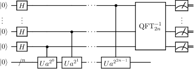
Next is the period-finding subroutine, the quantum part of Shor’s algorithm. We will use Quantum.NET to simulate the required quantum circuit, shown below:

The quantum circuit used in Shor's algorithm

Initializing the input and output quantum registers is as simple as it gets:

// 3. Pick m such that m = 2^l for some integer l and n² ≤ m < 2n².
int registerLength = ShorsAlgorithm.RegisterLength(n * n - 1);

// 4. Prepare two quantum registers in compound state |0⟩|0⟩. Let them be large enough to represent numbers up to m − 1, i.e. of length l.
QuantumRegister inputRegister = new QuantumRegister(0, registerLength);
QuantumRegister outputRegister = new QuantumRegister(0, registerLength);

// 3. Pick m such that m = 2^l for some integer l and n² ≤ m < 2n².

int registerLength = ShorsAlgorithm.RegisterLength(n * n - 1);

// 4. Prepare two quantum registers in compound state |0⟩|0⟩. Let them be large enough to represent numbers up to m − 1, i.e. of length l.

QuantumRegister inputRegister = new QuantumRegister(0, registerLength);

QuantumRegister outputRegister = new QuantumRegister(0, registerLength);

And so is applying the Hadamard transform to the first register:

// 5. Apply the Hadamard transform to the first register.
inputRegister = QuantumGate.HadamardGateOfLength(registerLength) * inputRegister;

1 2	// 5. Apply the Hadamard transform to the first register. inputRegister = QuantumGate.HadamardGateOfLength(registerLength) * inputRegister;

We use the following method to calculate $m$:

protected static int RegisterLength(int value)
{
	int length = 1;

	for (int bitCount = 16; bitCount > 0; bitCount /= 2)
	{
		if (value >= 1 << bitCount)
		{
			value >>= bitCount;
			length += bitCount;
		}
	}

	return length;
}

protected static int RegisterLength(int value)

{

int length = 1;

for (int bitCount = 16; bitCount > 0; bitCount /= 2)

{

if (value >= 1 << bitCount)

{

value >>= bitCount;

length += bitCount;

}

return length;

}

Another quick benchmark shows it to be about 3.6 times as fast as the equivalent approach using .NET’s logarithm, (int) Math.Log(n * n - 1, 2) + 1. It works by removing chunks of 16, 8, 4, 2 and 1 bit(s) (we’re working on 32-bit integers) when possible and counting the number of bits removed.

Now to the crux of Shor’s algorithm, but also the bottleneck in terms of runtime: modular exponentiation. We have to build a gate (more like a sub-circuit) that applies the map defined by $\left|x\right\rangle \left|0\right\rangle \rightarrow \left|x\right\rangle \left|a^x \bmod n\right\rangle$ to the full register.

Building such a circuit is a very complex matter and there are many approaches, but all start with a decomposition into modular multipliers. We use the fact that $a^x \bmod n$ $= \prod_{i=0}^{l-1} (a^{2^{i}} \bmod n)^{x_i} \bmod n$, where the $x_i$ are the bits of $x$ such that $x = \sum_{i=0}^{l-1} x_i 2^i$, to split the circuit into a series of controlled modular multiplication gates, each using a different qubit from the input register as a control qubit.

However, for the sake of simplicity, we will represent this circuit with a unique modular exponentiation gate. The map leaves the input registry unchanged, therefore it can be represented by a block diagonal matrix of total order $m^2$:

$\mathbf{M} = \begin{bmatrix}
\mathbf{M}_{0} & 0 & \cdots & 0 \\ 0 & \mathbf{M}_{1} & \cdots & 0 \\
\vdots & \vdots & \ddots & \vdots \\
0 & 0 & \cdots & \mathbf{M}_{m – 1}
\end{bmatrix}$

It also overrides the output registry regardless of its initial value (with the result of the modular exponentiation of the input registry), therefore the elements of $\mathbf{M}_{k}$ are $\mathbf{{m}_{k}}_{i, j} = 1$ if $i = a^k \bmod n$ and $0$ otherwise, regardless of $j$.

The resulting permutation matrix is built using the following:

protected static Matrix<Complex> ModularExponentiationMatrix(int n, int a, int registerLength)
{
	int matrixSize = 1 << (registerLength * 2);
	Matrix<Complex> modularExponentiationMatrix = Matrix<Complex>.Build.Sparse(matrixSize, matrixSize);

	int blockSize = 1 << registerLength;
	for (int i = 0; i < blockSize; i++)
	{
		int modularExponentiationResult = ShorsAlgorithm.ModIntPow(a, i, n);

		for (int j = 0; j < blockSize; j++)
		{
			modularExponentiationMatrix.At(i * blockSize + modularExponentiationResult, i * blockSize + j, 1);
		}
	}

	return modularExponentiationMatrix;
}

protected static Matrix<Complex> ModularExponentiationMatrix(int n, int a, int registerLength)

{

int matrixSize = 1 << (registerLength * 2);

Matrix<Complex> modularExponentiationMatrix = Matrix<Complex>.Build.Sparse(matrixSize, matrixSize);

int blockSize = 1 << registerLength;

for (int i = 0; i < blockSize; i++)

{

int modularExponentiationResult = ShorsAlgorithm.ModIntPow(a, i, n);

for (int j = 0; j < blockSize; j++)

{

modularExponentiationMatrix.At(i * blockSize + modularExponentiationResult, i * blockSize + j, 1);

}

return modularExponentiationMatrix;

}

Modular exponentiation is performed using a slightly modified version of exponentiation by squaring:

protected static int ModIntPow(int @base, int exponent, int modulus)
{
	int result = 1;

	while (exponent > 0)
	{
		if ((exponent & 1) == 1)
		{
			result = (result * @base) % modulus;
		}

		exponent >>= 1;
		@base = (@base * @base) % modulus;
	}

	return result;
}

protected static int ModIntPow(int @base, int exponent, int modulus)

{

int result = 1;

while (exponent > 0)

{

if ((exponent & 1) == 1)

{

result = (result * @base) % modulus;

}

exponent >>= 1;

@base = (@base * @base) % modulus;

}

return result;

}

We use the newly created permutation matrix to create a quantum gate we apply to the global register, formed from the input and output registers.

// 6. Apply a map defined by |x⟩ |0⟩ → |x⟩ |a^x mod n⟩.
Matrix<Complex> modularExponentiationMatrix = ShorsAlgorithm.ModularExponentiationMatrix(n, a, registerLength);
QuantumGate modularExponentiationGate = new QuantumGate(modularExponentiationMatrix);

QuantumRegister fullRegister = new QuantumRegister(inputRegister, outputRegister);

fullRegister = modularExponentiationGate * fullRegister;

// 6. Apply a map defined by |x⟩ |0⟩ → |x⟩ |a^x mod n⟩.

Matrix<Complex> modularExponentiationMatrix = ShorsAlgorithm.ModularExponentiationMatrix(n, a, registerLength);

QuantumGate modularExponentiationGate = new QuantumGate(modularExponentiationMatrix);

QuantumRegister fullRegister = new QuantumRegister(inputRegister, outputRegister);

fullRegister = modularExponentiationGate * fullRegister;

The registers are now entangled. The next step consists in applying the quantum Fourier transform to the input register, but it needs to be processed along with the output register in order to preserve entanglement. The solution consists in creating a quantum gate from two smaller ones: a quantum Fourier transform for the input register and an identity gate for the output register, which will be left unchanged.

// 7. Apply the quantum Fourier transform to the first register, which becomes 1/√m ∑(y=0...m−1) e^(2πxyi/m) |y⟩.
QuantumGate quantumFourierMatrixPlusIdentity = new QuantumGate(QuantumGate.QuantumFourierTransform(registerLength), QuantumGate.IdentityGateOfLength(registerLength));

fullRegister = quantumFourierMatrixPlusIdentity * fullRegister;

// 7. Apply the quantum Fourier transform to the first register, which becomes 1/√m ∑(y=0...m−1) e^(2πxyi/m) |y⟩.

QuantumGate quantumFourierMatrixPlusIdentity = new QuantumGate(QuantumGate.QuantumFourierTransform(registerLength), QuantumGate.IdentityGateOfLength(registerLength));

fullRegister = quantumFourierMatrixPlusIdentity * fullRegister;

It is now time to observe the first register so that it collapses into a pure state, and read its value. fullRegister is of length 2 * registerLength, so we use the portionStart and portionLength parameters of QuantumRegister.GetValue to only read the first registerLength bits, returning a value $y$:

// 8. Observe the first register.
fullRegister.Collapse(this.Random);

int inputRegisterValue = fullRegister.GetValue(0, registerLength);

// 8. Observe the first register.

fullRegister.Collapse(this.Random);

int inputRegisterValue = fullRegister.GetValue(0, registerLength);

The idea is now to perform continued fraction expansion on $y / m$. As explained above, the denominator of the fraction approximation is likely to be the period $p$ or a factor of it.

// 9. Perform continued fraction expansion on y/m to approximate it to k/p′ with p′ < n. The denominator p′ is therefore likely to be the period p or a factor of it.
float ratio = (float) inputRegisterValue / (1 << registerLength);

int denominator = ShorsAlgorithm.Denominator(ratio, n);

// 9. Perform continued fraction expansion on y/m to approximate it to k/p′ with p′ < n. The denominator p′ is therefore likely to be the period p or a factor of it.

float ratio = (float) inputRegisterValue / (1 << registerLength);

int denominator = ShorsAlgorithm.Denominator(ratio, n);

Every irrational number can be represented in precisely one way as an infinite continued fraction, which is an expression of the form:

$a_0 + \frac{1}{a_1 + \frac{1}{a_2 + \frac{1}{a_3 + {_\ddots}}}}$

Limiting the expression to a certain number of terms gives rational approximations called the convergents of the continued fraction. They are $a_0 = \frac{a_0}{1}$, $a_0 + \frac{1}{a_1} = \frac{a_1 a_0 + 1}{a_1 }$, $a_0 + \frac{1}{a_1 + \frac{1}{a_2}} = \frac{a_2 (a_1 a_0 + 1) + a_0}{a_2 a_1 + 1}$, and can generally be expressed as $\frac{h_n}{k_n}$, with the numerators and denominators recursively defined by $h_n = a_n h_{n − 1} + h_{n − 2}$ and $k_n = a_n k_{n − 1} + k_{n − 2}$.

This property allows us to find the greatest denominator $p’$ such that$p’ < n$, using the following implementation:

protected static int Denominator(float realNumber, int maximum)
{
	if (realNumber == 0f)
	{
		return 1;
	}

	int coefficient = 0;
	float remainder = realNumber;

	int[] previousNumerators = new int[] { 0, 1 };
	int[] previousDenominators = new int[] { 1, 0 };
	
	while (remainder != Math.Floor(remainder))
	{
		coefficient = (int) remainder;
		try { remainder = checked(1f / (remainder - coefficient)); } catch (System.OverflowException) { return previousDenominators[1]; }

		int numerator = coefficient * previousNumerators[1] + previousNumerators[0];
		int denominator = coefficient * previousDenominators[1] + previousDenominators[0];

		if (denominator >= maximum)
		{
			return previousDenominators[1];
		}

		previousNumerators[0] = previousNumerators[1];
		previousDenominators[0] = previousDenominators[1];
		previousNumerators[1] = numerator;
		previousDenominators[1] = denominator;
	}
	
	return previousDenominators[1];
}

protected static int Denominator(float realNumber, int maximum)

{

if (realNumber == 0f)

{

return 1;

}

int coefficient = 0;

float remainder = realNumber;

int[] previousNumerators = new int[] { 0, 1 };

int[] previousDenominators = new int[] { 1, 0 };

while (remainder != Math.Floor(remainder))

{

coefficient = (int) remainder;

try { remainder = checked(1f / (remainder - coefficient)); } catch (System.OverflowException) { return previousDenominators[1]; }

int numerator = coefficient * previousNumerators[1] + previousNumerators[0];

int denominator = coefficient * previousDenominators[1] + previousDenominators[0];

if (denominator >= maximum)

{

return previousDenominators[1];

}

previousNumerators[0] = previousNumerators[1];

previousDenominators[0] = previousDenominators[1];

previousNumerators[1] = numerator;

previousDenominators[1] = denominator;

}

return previousDenominators[1];

}

Now we have a candidate for $p$, we verify if $p’$ or one of its multiples is the period we’re looking for.

// 10. and 11. Verify that a^p′ ≡ 1 mod n. Otherwise, try the same thing with multiples of p′.
for (int period = denominator; period < n; period += denominator)
{
	//if (ShorsAlgorithm.IntPow(a, period) % n == 1)
	if (ShorsAlgorithm.ModIntPow(a, period, n) == 1)
	{
		return period;
	}
}

// 10. and 11. Verify that a^p′ ≡ 1 mod n. Otherwise, try the same thing with multiples of p′.

for (int period = denominator; period < n; period += denominator)

{

//if (ShorsAlgorithm.IntPow(a, period) % n == 1)

if (ShorsAlgorithm.ModIntPow(a, period, n) == 1)

{

return period;

}

If that’s the case, then we are done with the period-finding subroutine, and Shor’s algorithm as a whole. If not, we start the subroutine over:

// 12. Otherwise, go back to step 4.
return this.Period(n, a);

1 2	// 12. Otherwise, go back to step 4. return this.Period(n, a);

This article now comes to an end. We have successfully modeled Shor’s algorithm, and while it won’t help us factor anything (the classical alternatives being incomparably faster than simulating a system whose complexity grows exponentially with regard to the size of the input), it provides us with great insight as to how the algorithm can be implemented in practice.

RSA is not broken yet.

No, objects are not automatically passed by reference

While it makes sense for PHP beginners to first learn that objects are passed by reference rather than focus on technical details they need not comprehend yet, it worries me how many experienced developers still hold this belief.

The basic example used to justify said misconception is the following:

class MyClass {
	public $prop = 'foo';
}
 
function func($arg) {
	$arg->prop = 'bar';
}
 
$object = new MyClass;
echo $object->prop; // prints 'foo'
func($object);
echo $object->prop; // prints 'bar'

class MyClass {

public $prop = 'foo';

}

function func($arg) {

$arg->prop = 'bar';

}

$object = new MyClass;

echo $object->prop; // prints 'foo'

func($object);

echo $object->prop; // prints 'bar'

The function func has its sole argument passed by value, yet it somehow changed the state of $object. Is that not what passing by reference does?

Well, not exactly. Consider the following, where the object is replaced with a new one inside the function:

function func($arg) {
	$arg = new MyClass;
	$arg->prop = 'bar';
}
 
$object = new MyClass;
echo $object->prop; // prints 'foo'
func($object);
echo $object->prop; // still prints 'foo'

function func($arg) {

$arg = new MyClass;

$arg->prop = 'bar';

}

$object = new MyClass;

echo $object->prop; // prints 'foo'

func($object);

echo $object->prop; // still prints 'foo'

Here, $object remains unchanged. However, if we add a reference:

function func(&$arg) {
	$arg = new MyClass;
	$arg->prop = 'bar';
}
 
$object = new MyClass;
echo $object->prop; // prints 'foo'
func($object);
echo $object->prop; // prints 'bar' again

function func(&$arg) {

$arg = new MyClass;

$arg->prop = 'bar';

}

$object = new MyClass;

echo $object->prop; // prints 'foo'

func($object);

echo $object->prop; // prints 'bar' again

We now revert to the original behavior.

Now it has been shown that references do make a difference for objects, the best way to understand why is to clearly define both.

A reference, first, is nothing but an alias, which means that both variables point to the same location in memory and can therefore be used interchangeably.

An object variable, on the other hand, doesn’t contain the object itself but an identifier that allows the runtime to access its content. In fact, it works exactly like pointers in C++, and therefore explains PHP’s use of the same syntax as the ‘member of pointer’ operator (->), which translates to ‘point to the given property for the object of given identifier’.

What happens in the first example is that this identifier is passed by value and copied to $arg in the function scope. Then, the runtime is asked to modify the property prop of the object corresponding to the identifier. The variable $object in the global scope was never modified, but the object it points to was.

In the second example, the identifier is once again passed by value, but then, the local variable $arg is overridden with another identifier to another object, and it is the property prop of that second object that is modified, explaining why the original one remains unchanged.

The third example, finally, has the identifier passed by reference to func. A second object is once again created, and its identifier is saved in the alias $arg, which is, by definition, just another way to refer to the variable $object in the global scope, which in turn now points to a new, modified object.

Back to pointers to objects in C++, the code below shows how they can be used to obtain the exact same behavior as PHP objects:

#include <iostream>
#include <string>

using namespace std;

class MyClass {
public:
	MyClass() {
		this->prop = "foo";
	}

	string prop;
};

void func1(MyClass* arg) {
	arg = new MyClass;
	arg->prop = "bar";
}

void func2(MyClass* &arg) {
	arg = new MyClass;
	arg->prop = "bar";
}

int main()
{
	MyClass* object1 = new MyClass;
	cout << object1->prop << endl; // prints 'foo'
	func1(object1);
	cout << object1->prop << endl; // still prints 'foo'

	MyClass* object2 = new MyClass;
	cout << object2->prop << endl; // prints 'foo'
	func2(object2);
	cout << object2->prop << endl; // prints 'bar' again

	return 0;
}

#include <iostream>

#include <string>

using namespace std;

class MyClass {

public:

MyClass() {

this->prop = "foo";

}

string prop;

};

void func1(MyClass* arg) {

arg = new MyClass;

arg->prop = "bar";

}

void func2(MyClass* &arg) {

arg = new MyClass;

arg->prop = "bar";

}

int main()

{

MyClass* object1 = new MyClass;

cout << object1->prop << endl; // prints 'foo'

func1(object1);

cout << object1->prop << endl; // still prints 'foo'

MyClass* object2 = new MyClass;

cout << object2->prop << endl; // prints 'foo'

func2(object2);

cout << object2->prop << endl; // prints 'bar' again

return 0;

}

Though, if you know how pointers work, you probably didn’t need to read this article anyway.

In C#, the behavior is once again the same, but the introduction of reference types (variables that store references to their data, as opposed to directly containing the data) abstracts the concept of pointers and allows us to use objects directly, and with the ‘member of’ operator (.) only:

using System;

class MyClass
{
	public string prop = "foo";
}

class Program
{
	static void func1(MyClass arg)
	{
		arg = new MyClass();
		arg.prop = "bar";
	}

	static void func2(ref MyClass arg)
	{
		arg = new MyClass();
		arg.prop = "bar";
	}

	static void Main(string[] args)
	{
		MyClass object1 = new MyClass();
		Console.WriteLine(object1.prop); // prints 'foo'
		func1(object1);
		Console.WriteLine(object1.prop); // still prints 'foo'

		MyClass object2 = new MyClass();
		Console.WriteLine(object2.prop); // prints 'foo'
		func2(ref object2);
		Console.WriteLine(object2.prop); // prints 'bar' again
	}
}

using System;

class MyClass

{

public string prop = "foo";

}

class Program

{

static void func1(MyClass arg)

{

arg = new MyClass();

arg.prop = "bar";

}

static void func2(ref MyClass arg)

{

arg = new MyClass();

arg.prop = "bar";

}

static void Main(string[] args)

{

MyClass object1 = new MyClass();

Console.WriteLine(object1.prop); // prints 'foo'

func1(object1);

Console.WriteLine(object1.prop); // still prints 'foo'

MyClass object2 = new MyClass();

Console.WriteLine(object2.prop); // prints 'foo'

func2(ref object2);

Console.WriteLine(object2.prop); // prints 'bar' again

}

Please note that C# actually supports pointers (to value types and other pointer types), though they should only be used to interact with native functions or in performance-critical code.

Quantum.NET v1.1.0 is now available

Version 1.1.0 of Quantum.NET has been released today. It introduces several new features aimed at facilitating the building of more complex quantum circuits and the obtaining of the results they yield.

First is the introduction of identity gates:

QuantumGate.IdentityGate
QuantumGate.IdentityGateOfLength(int registerLength)

While useless in themselves, they become very powerful when combined with another new feature, quantum gate stacking, or the creation of quantum gates from other, smaller quantum gates (variadic constructor, also works with QuantumGate[] and IEnumerable<QuantumGate>):

QuantumGate quantumGate = new QuantumGate(QuantumGate.PauliZGate, QuantumGate.IdentityGate); // This gate will apply the Pauli-Z gate to the first qubit and leave the second one unchanged

1	QuantumGate quantumGate = new QuantumGate(QuantumGate.PauliZGate, QuantumGate.IdentityGate); // This gate will apply the Pauli-Z gate to the first qubit and leave the second one unchanged

This allows to apply a gate to a subsection of a quantum register, leaving the rest unchanged while preserving entanglement.

Another new feature is the reading of the values contained in pure-state quantum registers. Once an algorithm is run, we will be left with a register to observe which, once collapsed, will contain the data we need. Optional offset and length parameters can be used to read a subsection of the quantum register only, as often required.

QuantumRegister quantumRegister = new QuantumRegister(27); // |11011>
int a = quantumRegister.GetValue(); // 27 (0b11011)
int b = quantumRegister.GetValue(1); // 11 (0b1011)
int c = quantumRegister.GetValue(1, 3); // 5 (0b101)
int d = Qubit.EPRPair.GetValue(); // cannot be used on a mixed state; throws System.SystemException

QuantumRegister quantumRegister = new QuantumRegister(27); // |11011>

int a = quantumRegister.GetValue(); // 27 (0b11011)

int b = quantumRegister.GetValue(1); // 11 (0b1011)

int c = quantumRegister.GetValue(1, 3); // 5 (0b101)

int d = Qubit.EPRPair.GetValue(); // cannot be used on a mixed state; throws System.SystemException

Quantum.NET is available as a NuGet package under Lachesis.QuantumComputing, and the source code can be found on GitHub at phbaudin/quantum-computing.

Quantum.NET: a new quantum computing library in C#

I’ve just published the first version of my latest project, a quantum computing library in C# called Quantum.NET that allows the manipulation of qubits and the modeling of quantum circuits.

It is available as a NuGet package under Lachesis.QuantumComputing, and the source code can be found on GitHub at phbaudin/quantum-computing.

The way it works is pretty straightforward. A qubit can be created from its probability amplitudes:

Qubit qubit = new Qubit(Complex.One / Math.Sqrt(2), Complex.ImaginaryOne / Math.Sqrt(2)); // (|0> + i |1>) / √2

1	Qubit qubit = new Qubit(Complex.One / Math.Sqrt(2), Complex.ImaginaryOne / Math.Sqrt(2)); // (\|0> + i \|1>) / √2

Or from its amplitudes’ real and imaginary parts:

Qubit qubit = new Qubit(1 / Math.Sqrt(2), 0, 0, 1 / Math.Sqrt(2)); // (|0> + i |1>) / √2

1	Qubit qubit = new Qubit(1 / Math.Sqrt(2), 0, 0, 1 / Math.Sqrt(2)); // (\|0> + i \|1>) / √2

It can also be created from its colatitude and longitude on the Bloch sphere:

Qubit qubit = new Qubit(Math.PI / 2, 0); // (|0> + |1>) / √2

1	Qubit qubit = new Qubit(Math.PI / 2, 0); // (\|0> + \|1>) / √2

Shortcuts are available for notable qubits:

Qubit zero = Qubit.Zero; // |0>
Qubit one = Qubit.One; // |1>

1 2	Qubit zero = Qubit.Zero; // \|0> Qubit one = Qubit.One; // \|1>

A qubit is a quantum register of length 1 and can be manipulated as such. The Qubit class is merely a subclass of QuantumRegister designed for ease of use:

QuantumRegister quantumRegister = Qubit.Zero;

1	QuantumRegister quantumRegister = Qubit.Zero;

Shortcuts are also available for notable quantum registers:

QuantumRegister EPRPair = QuantumRegister.EPRPair; // (|00> + |11>) / √2 (Einstein–Podolsky–Rosen pair)
QuantumRegister WState = QuantumRegister.WState; // (|001> + |010> + |100>) / √3 (W state)
QuantumRegister WState4 = QuantumRegister.WStateOfLength(4); // (|0001> + |0010> + |0100> + |1000>) / 2 (generalized W state for 4 qubits)
QuantumRegister GHZState = QuantumRegister.GHZState; // (|000> + |111>) / √2 (simplest Greenberger–Horne–Zeilinger state)
QuantumRegister GHZState4 = QuantumRegister.GHZStateOfLength(4); // (|0000> + |1111>) / √2 (GHZ state for 4 qubits)

QuantumRegister EPRPair = QuantumRegister.EPRPair; // (|00> + |11>) / √2 (Einstein–Podolsky–Rosen pair)

QuantumRegister WState = QuantumRegister.WState; // (|001> + |010> + |100>) / √3 (W state)

QuantumRegister WState4 = QuantumRegister.WStateOfLength(4); // (|0001> + |0010> + |0100> + |1000>) / 2 (generalized W state for 4 qubits)

QuantumRegister GHZState = QuantumRegister.GHZState; // (|000> + |111>) / √2 (simplest Greenberger–Horne–Zeilinger state)

QuantumRegister GHZState4 = QuantumRegister.GHZStateOfLength(4); // (|0000> + |1111>) / √2 (GHZ state for 4 qubits)

A quantum register can be created from other quantum registers (variadic constructor, also works with QuantumRegister[] and IEnumerable<QuantumRegister>):

QuantumRegister quantumRegister = new QuantumRegister(Qubit.Zero, QuantumRegister.EPRPair); // (|000> + |011>) / √2

1	QuantumRegister quantumRegister = new QuantumRegister(Qubit.Zero, QuantumRegister.EPRPair); // (\|000> + \|011>) / √2

Or from the 2ⁿ complex probability amplitudes of each of its pure states (variadic constructor, also works with Complex[] and IEnumerable<Complex>):

QuantumRegister quantumRegister = new QuantumRegister(0, 1 / Math.Sqrt(2), 1 / Math.Sqrt(2), 0); // (|01> + |10>) / √2
QuantumRegister error = new QuantumRegister(0, 1, 0); // the number of amplitudes is not a power of 2; throws System.ArgumentException

1 2	QuantumRegister quantumRegister = new QuantumRegister(0, 1 / Math.Sqrt(2), 1 / Math.Sqrt(2), 0); // (\|01> + \|10>) / √2 QuantumRegister error = new QuantumRegister(0, 1, 0); // the number of amplitudes is not a power of 2; throws System.ArgumentException

Quantum registers are mostly used to represent numbers and can therefore be created from integers (this will naturally generate pure states):

QuantumRegister seven = new QuantumRegister(7); // |111>
QuantumRegister threeOnThreeBits = new QuantumRegister(3, 3); // |011>

1 2	QuantumRegister seven = new QuantumRegister(7); // \|111> QuantumRegister threeOnThreeBits = new QuantumRegister(3, 3); // \|011>

A quantum register can be observed and collapse into a pure state (note: use your own Random instance to avoid issues with pseudorandom number generator determinism):

Random random = new Random();
QuantumRegister quantumRegister = QuantumRegister.EPRPair;
quantumRegister.Collapse(random); // |00> or |11>

Random random = new Random();

QuantumRegister quantumRegister = QuantumRegister.EPRPair;

quantumRegister.Collapse(random); // |00> or |11>

Quantum gates are required to operate on quantum registers. Shortcuts are also available for notable quantum gates:

QuantumGate.HadamardGate
QuantumGate.HadamardGateOfLength(int registerLength)
QuantumGate.NotGate
QuantumGate.PauliYGate
QuantumGate.PauliZGate
QuantumGate.SquareRootNotGate
QuantumGate.PhaseShiftGate(double phase)
QuantumGate.SwapGate
QuantumGate.SquareRootSwapGate
QuantumGate.ControlledNotGate
QuantumGate.ControlledGate(QuantumGate gate)
QuantumGate.ToffoliGate
QuantumGate.FredkinGate
QuantumGate.QuantumFourierTransform(int registerLength)

Quantum gates can also be created from a bidimensional array of complex numbers:

QuantumGate quantumGate = new QuantumGate(new Complex[,] {
	{ 1, 1 },
	{ 1, 0 },
});

QuantumGate quantumGate = new QuantumGate(new Complex[,] {

{ 1, 1 },

{ 1, 0 },

});

Applying a quantum gate to a quantum register is as simple as using the multiplication operator on them:

QuantumRegister quantumRegister = Qubit.Zero; // |0>
quantumRegister = QuantumGate.HadamardGate * quantumRegister; // (|0> + |1>) / √2
quantumRegister = QuantumGate.HadamardGate * quantumRegister; // |0>
quantumRegister = QuantumGate.NotGate * quantumRegister; // |1>

QuantumRegister quantumRegister = Qubit.Zero; // |0>

quantumRegister = QuantumGate.HadamardGate * quantumRegister; // (|0> + |1>) / √2

quantumRegister = QuantumGate.HadamardGate * quantumRegister; // |0>

quantumRegister = QuantumGate.NotGate * quantumRegister; // |1>

Unary gates only operate on one qubit, binary gates on two, etc.:

QuantumRegister error = QuantumGate.PauliYGate * QuantumRegister.EPRPair; // a unary gate cannot be applied to two qubits; throws System.ArgumentException

1	QuantumRegister error = QuantumGate.PauliYGate * QuantumRegister.EPRPair; // a unary gate cannot be applied to two qubits; throws System.ArgumentException

Please note that this is not a literal arithmetic library. While measures have been taken to circumvent a range of errors caused by floating-point precision, the use of QuantumRegister.AlmostEquals might be required in places:

QuantumRegister almostOne = new Qubit(Complex.One, Math.Cos(Math.PI / 2) * Complex.One);
QuantumRegister one = new Qubit(Complex.One, 0);
almostOne.AlmostEquals(one); // true

QuantumRegister almostOne = new Qubit(Complex.One, Math.Cos(Math.PI / 2) * Complex.One);

QuantumRegister one = new Qubit(Complex.One, 0);

almostOne.AlmostEquals(one); // true

Hope you find this useful!